Thermal Engineering

Explore the mechanics behind geyser eruptions, focusing on fluid dynamics, phase transitions, and thermal energy in natural environments.

How Do Geysers Erupt Through Fluid Dynamics?

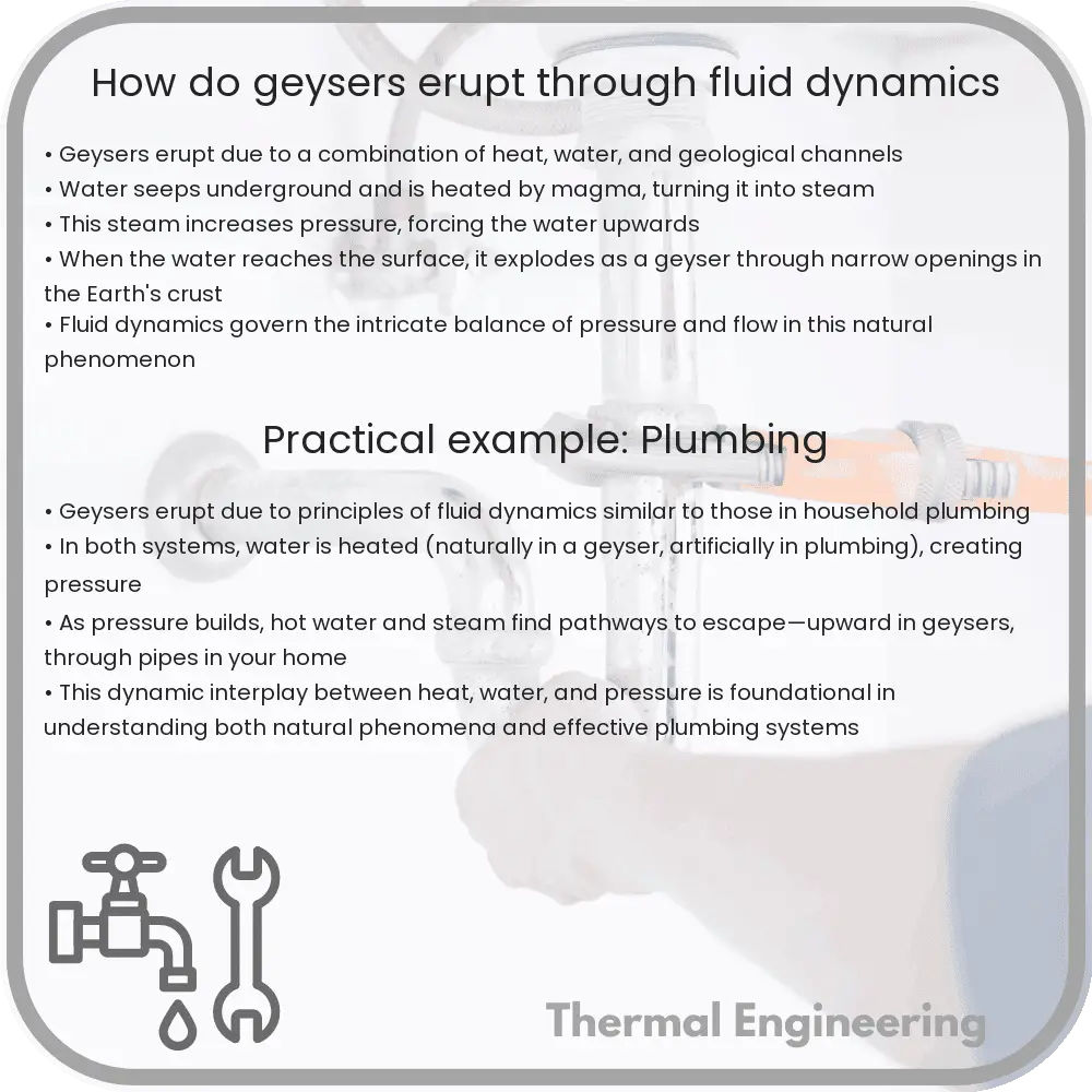
Geysers are natural phenomena that create spectacular eruptions of water and steam. Understanding how these eruptions occur requires an exploration of fluid dynamics, a branch of physics concerned with the movement of fluids. Geysers provide a fascinating case study of phase transitions and pressure changes in confined environments.

The Mechanics of a Geyser

A geyser’s activity hinges on its unique underground structure, which typically includes a tight network of fractures and cavities within rock. These subterranean chambers are key to the mechanics of geyser eruption, operating under principles of thermodynamics and hydrogeology.

Heat Source

At the base of a geyser’s operation is a heat source, usually geothermal energy derived from Earth’s internal heat. This heat warms nearby water reservoirs trapped in porous rock or caverns deep underground.

Water Heating and Steam Accumulation

As water at the bottom of the geyser’s chamber heats up, it begins to expand. Since the water is confined within rock structures, it cannot expand freely and thereby increases in pressure. This process continues until the water’s temperature exceeds its standard boiling point, a phenomenon possible due to the overlying water’s pressure, which increases the boiling point in a process known as boiling point elevation.

Phase Transition and Eruption

• Initiation: When water converts into steam, its volume expands dramatically — approximately by a factor of 1,600. This sudden increase in volume creates a surge in pressure.
• Pressure Release: As pressure builds, less heated water at the top of the column can begin to percolate to the surface, releasing some pressure.
• Steam Explosions: Once the pressure is sufficiently diminished, the superheated water at the bottom, now able to rapidly transform into steam, quickly ascends, carrying water with it in a powerful rush upwards. This phase transition is abrupt and violent, leading to the majestic eruption observed at the surface.

The Role of Surrounding Temperature

External conditions, particularly air temperature and pressure, have significant impacts on the timing and intensity of geyser eruptions. Colder air can increase the eruption’s visibility due to greater condensation of the steam phase into water droplets.

Mathematical Perspective

Understanding geyser eruptions can also be approached mathematically by considering energy conservation and fluid dynamics equations. The basic energy equation could be posed as:

1. mC_p(dT/dt) = Q – P, where:
2. m is mass of the water,
3. C_p is the specific heat at constant pressure,
4. Q is the heat added,
5. P is the power associated with pressure work,
6. dt is the change in temperature over time.

This simplified model can help explain the conditions under which the water transitions to steam leading up to an eruption.

Conclusion

Geysers are a dramatic demonstration of nature’s power and the complexities of fluid dynamics. The processes of heating, phase change, pressure dynamics, and sudden release encapsulate fascinating physical principles that yield their awe-inspiring eruptions. Such natural wonders provide not only a visual spectacle but a significant educational resource for understanding Earth’s geothermal activities and the physics behind them.

Learn about the Eckert number in fluid dynamics, a dimensionless parameter crucial for analyzing heat transfer in high-speed fluid flows.

Understanding the Eckert Number in Fluid Dynamics

In fluid dynamics, the Eckert number is a dimensionless number that describes the ratio of kinetic energy to enthalpy in a fluid flow. It is particularly useful in analyzing flows where significant heat transfer occurs due to compression or friction, such as in high-speed aerodynamics and some types of heat exchangers.

Definition and Formula

The Eckert number (Ec) is defined as the ratio of the fluid’s kinetic energy to its enthalpy change, represented by the formula:

\[ \text{Ec} = \frac{V^2}{c_p \Delta T} \]

where:

• \( V \) is the characteristic velocity of the fluid,
• \( c_p \) is the specific heat capacity of the fluid at constant pressure,
• \( \Delta T \) is the temperature difference driving heat transfer.

This formula highlights how faster fluid movements (higher \( V \)) or lower heat capacities and temperature differences lead to higher Eckert numbers, signifying the dominance of kinetic energy in the system’s dynamics.

Physical Significance

The Eckert number is particularly significant in scenarios where thermal energy conversion is critical. A higher Eckert number indicates that the mechanical energy (kinetic) is large compared to the thermal energy, suggesting that effects like viscous heating can be important. Such conditions are often encountered in high-speed aerodynamics, where the speed of the fluid makes convective heat transfer a major factor.

On the other hand, a low Eckert number indicates that kinetic energies are small in comparison to the energy changes due to heat transfer, typical in many low-speed fluid flows in heat exchangers or in natural convection scenarios.

Applications in Engineering

Engineers use the Eckert number to:

• Analyze heat transfer in high-speed flows such as those found around aircraft or in gas turbines,
• Assess the significance of viscous dissipation in fluid flows,
• Design more effective cooling systems in engines and other mechanical systems where heat transfer and fluid dynamics interplay significantly.

Conclusion

The Eckert number serves as a vital dimensionless parameter in fluid dynamics, facilitating the understanding and prediction of heat transfer characteristics in fluid flows. By quantifying the relative influence of kinetic and thermal energies, it aids engineers in optimizing system performance across a variety of applications where speed and heat interact closely.

Exploring recent advancements in heat pipe technology and its applications in electronics cooling, aerospace, and renewable energy sectors.

Advancements in Heat Pipe Technology

Heat pipe technology is an essential component in modern heat management systems, offering superior heat transport capabilities. As industries and technologies advance, the development of more efficient and versatile heat pipes has become crucial. This article explores recent advancements in heat pipe technology, emphasizing their impact on electronics cooling, aerospace, and renewable energy sectors.

Enhancements in Heat Pipe Materials and Design

One of the significant advancements in heat pipe technology is the development of new materials and designs. Traditionally, heat pipes were predominantly made of copper and aluminum due to their excellent thermal conductivity. However, recent research has focused on using composite materials or adding nanoparticles to the working fluid, significantly enhancing the thermal performance.

• Composite Materials: By integrating materials like carbon fiber or graphene, heat pipes can achieve better structural strength and improved thermal conductivity, which is crucial for aerospace applications where weight and durability are critical.
• Nanofluids: Adding nanoparticles to the working fluid inside the heat pipe has shown to increase the effective thermal conductivity and the heat transfer coefficient. These particles increase the effective surface area and the thermal conduction capability of the fluid, enhancing the overall efficiency of heat pipes.

Variable Conductance Heat Pipes (VCHPs)

Variable Conductance Heat Pipes offer a dynamic response to varying thermal loads, making them particularly useful in applications where the heat load fluctuates significantly, such as in satellites and space vehicles. VCHPs adjust their effective thermal conductance in response to changing conditions, preventing the temperature of sensitive components from fluctuating excessively.

Applications in Renewable Energy

Heat pipes play a critical role in improving the efficiency of renewable energy systems. In solar power systems, heat pipes are used to transport heat from solar collectors to water tanks or power conversion devices efficiently. This technology has also been adapted for use in geothermal energy systems, where it helps in transferring heat from the earth’s core to the surface more effectively.

Advancements in Electronics Cooling

As electronic devices become increasingly powerful and compact, managing waste heat effectively has grown crucial. Advances in heat pipe technology have led to the development of ultra-thin heat pipes, which are perfect for use in smartphones, laptops, and other portable electronic devices. These thin pipes provide an effective means for heat dissipation without contributing significantly to the weight or thickness of the device.

• Loop Heat Pipes (LHPs): A sophisticated variant of the traditional heat pipe, Loop Heat Pipes are extensively used in high heat flux applications in both aerospace and consumer electronics. LHPs are capable of operating against gravity, making them ideal for spacecraft and vertical-mount applications in consumer electronics.

Future Prospects

The future of heat pipe technology looks promising, driven by ongoing research aimed at improving their efficiency and adaptability. New areas, such as the use of heat pipes in electric vehicle battery cooling systems and integrating them with IoT devices for smart thermal management, are likely to be important growth avenues. Moreover, continuous improvements in materials science and fluid dynamics are expected to unlock even more applications, reinforcing the role of heat pipes in modern engineering.

In conclusion, the advancements in heat pipe technology are revolutionizing multiple industries by improving efficiency and allowing for more compact and robust designs. As research progresses, we can anticipate broader applications and enhancements that will continue to push the boundaries of what is possible in heat management systems.

Learn how peristaltic pumps work, their applications in industries like medical and food processing, and advantages like preventing contamination.

Understanding the Mechanics of Peristaltic Pumps

Peristaltic pumps, often used in medical applications, laboratories, and food processing, employ a unique mechanism to move fluids without any contact between the fluid and the pump mechanism. This not only ensures the purity of the fluid but also enables the transportation of viscous, abrasive, or sensitive substances. Let’s explore how these devices function and their key components.

Basic Design and Operation

A peristaltic pump typically consists of a flexible tube fitted inside a circular pump casing. The rotary mechanism of the pump includes rollers or shoes that compress the tube as they rotate, creating a wave of constriction that travels along the length of the tube. This action mimics the natural peristaltic movements found in biological systems, such as the gastrointestinal tract, which is how this type of pump gets its name.

The Peristaltic Motion

The operation of a peristaltic pump is divided into several key phases:

• Compression: As the rotor turns, the rollers push against the flexible tube, flattening it. This compression blocks the flow of fluid at this point.
• Occlusion: Continued rotation moves the blockage forward, effectively pushing the fluid within the tube ahead of the roller.
• Release and Replenishment: Once the roller passes, the tube’s elasticity (typically made from materials like silicone or Tygon) causes it to regain its original shape, creating a vacuum. This vacuum pulls more fluid into the tube, preparing for the next cycle.

This continuous process of squeezing and releasing the tube moves the fluid in a smooth, consistent manner, which is advantageous for dosing and precision tasks.

Advantages of Peristaltic Pumps

Peristaltic pumps present several distinct advantages:

• No Contamination: The fluid only contacts the inside of the tube, eliminating the risk of contamination from the pump mechanism.
• Low Maintenance: The simplicity of the design means fewer moving parts to maintain or replace beyond the tube.
• Handling of Viscous Fluids: Performs well with thick or viscous substances, as the fluid does not need to fill the entire pumping chamber.
• Reversible: By simply reversing the direction of rotation, peristaltic pumps can easily reverse the flow of fluids, useful for filling/dispensing and sampling applications.

The ability to handle a wide range of fluids, coupled with its simplicity in design and operation, makes the peristaltic pump a versatile and robust tool for various applications across different industries.

Applications of Peristaltic Pumps

Due to their unique characteristics, peristaltic pumps are widely used in several fields:

• Medical: For dosing drugs or nutrients where precise volume control is necessary and contamination could have severe consequences.
• Laboratory: In research environments where cross-contamination between samples must be avoided.
• Food Processing: They are employed in the handling of food products, ensuring a sterile environment and maintaining the integrity of delicate ingredients.
• Chemical Processing: Useful for pumping harmful chemicals as the pump’s mechanics are never exposed to the chemical.

The versatility of peristaltic pumps makes them indispensable in scenarios requiring high levels of sanitation, precise flow control, and the safe handling of sensitive or harsh substances.

Conclusion

Peristaltic pumps blend simplicity, efficiency, and precision, making them an essential component in numerous applications where fluid integrity and purity are paramount. Their ability to replicate a natural biological process mechanically is a perfect example of engineering inspired by nature, providing solutions that are both ingenious and effective.

Explore how the Kelvin-Helmholtz Instability manifests in fluid dynamics through velocity shear between differing fluid densities.

Understanding the Kelvin-Helmholtz Instability

The Kelvin-Helmholtz instability (KHI) is a fluid dynamics phenomenon that occurs when there is velocity shear in a single continuous fluid, or at the interface between two different fluids. Named after Lord Kelvin and Hermann von Helmholtz, who first analyzed this instability in the 19th century, it is a common occurrence not just on Earth in oceans and atmospheric phenomena, but also in astrophysical contexts, such as in the atmospheres of other planets and the interstellar medium.

What Causes Kelvin-Helmholtz Instability?

Kelvin-Helmholtz Instability arises when there are two fluids of different densities moving at different velocities. The velocity difference leads to a shear force at the interface between the two fluids. For instance, consider a lighter fluid with velocity v₁ over a denser fluid moving with a slower velocity v₂. This velocity differential results in a tangential shear across the interface, potentially leading to the rolling up of the fluid interface into wave-like structures, commonly observed as cloud formations resembling ocean waves.

Mathematical Description of KHI

The stability of the interface can be studied by analyzing the perturbations (small disturbances) at the interface. The simplest mathematical approach involves using the incompressible inviscid flow assumptions whereby the dynamics are governed by the Rayleigh-Taylor instability condition. Mathematically, the criterion for the onset of the Kelvin-Helmholtz instability can be expressed as:

The growth rate, ω, of wave-like disturbances in the interface is given by:

ω² = (ρ₂ – ρ₁) * k * (v₁ – v₂)² / (ρ₂ + ρ₁)

where ρ₁ and ρ₂ are the densities of the two fluids, v₁ and v₂ are their respective velocities, and k is the wave number (related to the wavelength of the perturbation).

If ω² is positive, the interface is unstable and perturbations will grow exponentially, leading to the rolling, wave-like structures characteristic of Kelvin-Helmholtz instability.

Real-World Examples and Applications

• Atmospheric Sciences: The wavy clouds often seen on a windy day are a practical illustration of KHI, usually forming at altitudes where two streams of air move at different speeds.
• Oceanography: Internal waves in oceans, which impact marine structure and submarine navigation, often result from KHI due to differential movement of water layers.
• Astronomy: The bands and storms observed on planets such as Jupiter and Saturn, and even interactions in the solar wind, owe their behavior in part to KHI.
• Engineering: In mechanical and aerospace engineering, understanding and managing KHI is crucial for improving the aerodynamic efficiency and stability of structures subjected to different flow velocities.

In conclusion, the Kelvin-Helmholtz Instability not only provides captivating visual phenomena but also challenges engineers and scientists to better understand and predict the dynamics of fluids. As such, it holds significance across various branches of physical and applied sciences.

Learn about vortex shedding, a fluid dynamics phenomenon, and its engineering applications.

Understanding Vortex Shedding in Fluid Dynamics

Vortex shedding is a fascinating and complex phenomenon in fluid dynamics that occurs when a fluid such as air or water flows past a blunt object. The process is characterized by the formation of alternating vortices or swirling patterns on opposite sides of the object. This article will explore the principles behind vortex shedding, its implications in engineering, and how understanding it can lead to more efficient designs in various engineering fields.

Basic Principles of Vortex Shedding

When a fluid flows past an object, it can start to separate from the surface of the object at certain points along its boundary. This separation of flow creates a series of low-pressure vortices behind the object. The formation and subsequent shedding of these vortices occur alternately from one side of the object to the other, which can set up a vibrating pattern known as vortex shedding.

The frequency at which these vortices shed is described by the Strouhal number (St), a dimensionless number given by the equation:

St = f * D / V

• f is the frequency of vortex shedding
• D is the characteristic dimension (typically diameter) of the object
• V is the velocity of the fluid

The Strouhal number is crucial for predicting the shedding frequency and understanding the resulting flow patterns around blunt objects. This understanding helps engineers in designing structures that can withstand or minimize the effects of fluctuating forces due to vortex shedding.

Effects and Applications in Engineering

Vortex shedding is not just a theoretical concept; it has practical implications in engineering. Here are a few examples:

• Structural Engineering: In the construction of tall buildings or bridges, engineers must consider the effects of wind loads. Vortex shedding can induce oscillations in structures, which, if aligned with the structure’s natural frequency, could lead to structural failure due to resonance. The Tacoma Narrows Bridge collapse in 1940 is a famous example of such a failure.
• Aerospace Engineering: In aircraft design, engineers need to ensure that tail wings and other surfaces are capable of handling the stress caused by vortex shedding at various speeds and angles of attack.
• Marine Engineering: For offshore platforms and ship hulls, the patterns of vortex shedding must be analyzed to prevent vibrations which might lead to fatigue in the structural components.

Controlling Vortex Shedding

Given the potential adverse effects of uncontrolled vortex shedding, engineers have developed multiple strategies to manage or suppress it:

1. Vortex-Inducing Devices: Devices such as spoilers can be added to structures to alter the flow and reduce the formation of coherent vortices.
2. Shaping the Object: Streamlining objects to alter the flow separation points and reduce the lift coefficient can significantly mitigate vortex induced vibrations.
3. Tuning the Natural Frequency: By changing the stiffness or mass distribution of a structure, its natural frequency can be altered so it does not coincide with the frequency of vortex shedding.

Conclusion

Understanding vortex shedding is crucial for engineers across many industries. By applying this knowledge, engineers can design structures and devices that are safe, efficient, and less prone to the detrimental effects of fluid-structure interactions. The ongoing study of vortex shedding not only aids in improving existing designs but also inspires innovation in tackling new engineering challenges posed by complex fluid flows.

This basic introduction to the principles of vortex shedding in fluid dynamics illustrates its importance and applications. For engineers and designers, mastering this aspect of fluid mechanics is essential for optimizing performance and ensuring structural integrity in their projects.

Learn about Pascal’s Law in hydraulics, the principle explaining force transmission through fluids in hydraulic systems.

Understanding Pascal’s Law in Hydraulics

In the world of fluid mechanics, Pascal’s Law is a fundamental principle that plays a vital role in hydraulic systems. Named after Blaise Pascal, a French mathematician and physicist, this law provides the foundation for understanding how forces are transmitted through fluids. Let’s explore what Pascal’s Law is, how it works, and its applications in hydraulic systems.

What is Pascal’s Law?

Pascal’s Law states that when pressure is applied to a confined fluid, this pressure is transmitted undiminished throughout the fluid in all directions. The formal expression of Pascal’s Law is:

\( P = \frac{F}{A} \)

where:

• P is the pressure exerted on the fluid,
• F is the force applied, and
• A is the area on which the force is applied.

This means that any change in pressure applied at any point in a closed fluid is transmitted equally throughout the entirety of the fluid.

How Pascal’s Law Works in Hydraulics

Hydraulic systems utilize Pascal’s Law to perform work, such as lifting heavy loads or operating machinery. These systems consist essentially of two cylinders connected by a tube and filled with fluid—usually oil. Here’s how it applies:

• A force is applied to the fluid in a small piston, creating pressure.
• The pressure is transmitted undiminished through the fluid to all parts of the hydraulic system, including a larger piston.
• The larger piston, due to its larger area, then generates a larger force effectively multiplying the initial force applied.

The resulting multiplication of force is a key advantage in hydraulic systems, enabling them to perform tasks that would require much greater physical effort.

Application of Pascal’s Law in Real World

Hydraulic systems are found in a wide range of applications all around us. Some common examples include:

• Automotive Brakes: When a driver applies pressure to the brake pedal, this pressure is transmitted via brake fluid to apply the brakes at the wheels.
• Hydraulic Lifts: Used in various types of engineering machinery like forklifts and cherry pickers as well as in vehicle repair shops to lift heavy vehicles.
• Aircraft Hydraulics: Used in the control systems of most aircraft, hydraulic systems help in operations such as extending and retracting landing gears, operating control surfaces, and braking.

Conclusion

Pascal’s Law is a pivotal concept in fluid mechanics that is employed in designing various hydraulic devices. By understanding how pressure is transmitted in fluids, engineers can continue to create effective hydraulic systems that enhance our ability to perform work efficiently and safely. Whether it’s in automotive systems, industrial machines, or aircraft, the applications of Pascal’s Law demonstrate its importance in numerous engineering fields.

Through the understanding and application of such fundamental principles, we can harness the power of physics to develop technologies that significantly impact our daily lives and industries.

Learn how the Venturi Effect enhances fluid speed in constricted pipes, essential in engineering and technology applications.

Understanding the Venturi Effect in Fluid Flow

The Venturi effect is a fundamental and applied principle in fluid dynamics that describes how the velocity of a fluid increases as it passes through a constricted section of a pipe. This principle is named after the Italian physicist Giovanni Battista Venturi, who discovered the phenomenon in the late 18th century. Understanding this effect is essential in various engineering applications, ranging from carburetors in engines to measuring the flow rate of fluids in industrial processes.

How the Venturi Effect Works

When a fluid such as water or air flows through a pipe that has a narrow section, the flow speed of the fluid increases as it enters the constriction. This acceleration occurs because the fluid is forced to converge into a smaller area, reducing its pressure as per the principle of conservation of energy.

Mathematical Description of the Venturi Effect

The behavior of fluid flow through a Venturi tube can be described mathematically using the Bernoulli’s Equation and the Continuity Equation:

• Bernoulli’s Equation: This principle states that an increase in the speed of the fluid occurs simultaneously with a decrease in pressure or a decrease in the fluid’s potential energy. It is typically expressed as:

P₁ + 0.5ρv₁² + ρgh₁ = P₂ + 0.5ρv₂² + ρgh₂

• Continuity Equation: This equation asserts that the mass of the fluid that enters the tube must be equal to the mass exiting it. For an incompressible fluid, it implies that the product of the cross-sectional area (A) and the velocity (v) of the fluid remains constant:

A₁v₁ = A₂v₂

Applications of the Venturi Effect

The Venturi effect has practical applications in various fields of engineering and technology:

• Flow Measurement: Devices such as the Venturi meter are used to measure the flow rate of a fluid. By observing the pressure difference between the wider and the narrower sections of the tube, one can calculate the flow rate using the derived equations.
• Aerodynamics: In automotive and aviation industries, the Venturi effect is exploited to improve the performance of engines and aerodynamic structures, influencing design considerations.
• Medical Devices: Certain respiratory equipment and atomizers use this principle to control the flow of air and medicine.
• Environmental Engineering: Venturi scrubbers are employed to remove particulate matter from industrial exhaust by forcing it to contact water droplets.

The Venturi effect exemplifies how principles of physics are fundamental to engineering practices, providing efficiency and innovation across diverse applications. By leveraging the relationship between pressure, velocity, and flow area, engineers can design systems that are effective and optimized for specific needs.

Learn about the Coanda Effect, a key fluid dynamics phenomenon where fluids follow surface contours, influencing engineering design and technology.

Understanding the Coanda Effect in Fluids

The Coanda Effect is a fundamental concept in fluid dynamics, observed when a jet of fluid (which can be a liquid or a gas) attaches itself to a nearby surface and follows its contour. Named after Romanian inventor Henri Coanda, who first recognized and described this phenomenon in the early 20th century, the Coanda Effect has significant applications across various fields of engineering, including aerospace, mechanical, and civil engineering.

How the Coanda Effect Works

The basic principle underlying the Coanda Effect is that fluid molecules adhere to and travel along a surface due to the intrinsic properties of viscosity (the internal friction within the fluid) and the tendency to minimize energy expenditure. When a fluid is discharged from a nozzle or opening, it naturally seeks a path of least resistance. If a curved surface is placed close to the flow, the fluid’s inertia is insufficient to overcome the attraction to the surface, and thus it “clings” to it, following its shape.

Mathematically, this effect can be partly explained by Bernoulli’s principle, which states that an increase in the speed of the fluid occurs simultaneously with a decrease in pressure or potential energy. The higher velocity of the fluid along the contours of a surface results in lower pressure, which pulls the fluid towards the surface, helping it to stay attached.

Real-World Applications

• Aerospace Engineering: Airplane wings are designed to take advantage of the Coanda Effect. The curvature of the wing forces air to move faster over the top surface than the bottom, creating lift. Modern jet engines also use this effect to improve the efficiency of thrust.
• Automotive Engineering: The design of car bodies can incorporate aspects of the Coanda Effect to control the airflow around the vehicle, minimizing drag and improving fuel efficiency.
• Civil Engineering: The Coanda Effect is utilized in the design of roofs and structures to manage wind load and water drainage, ensuring that water flows in a controlled manner over surfaces.
• Environmental Engineering: This effect is applied in ventilation systems and in the design of equipment for pollutant removal from industrial emissions, enhancing the capture efficiency.

Exploring the Coanda Effect through Experiments

One simple experiment to observe the Coanda Effect involves a stream of water and a spoon. By holding the convex side of a spoon close to a thin stream of water, one can observe the water cling and follow the curve of the spoon. This illustrates how the flow is altered by the presence of a nearby surface, confirming the behavior predicted by the Coanda Effect.

Conclusion

Despite its seemingly simple nature, the Coanda Effect is a complex phenomenon that demonstrates the intricate behavior of fluids in motion. Its wide range of applications across various fields of engineering underscores its importance in design and innovation. Understanding this effect not only aids in comprehending fluid dynamics but also fuels advancements in technology and engineering design.

This exploratory journey into the Coanda Effect offers a glimpse into how fluids interact with surfaces, providing a foundational insight that is crucial for both students and professionals in the engineering realm.

Learn how fractal structures improve heat transfer in engineering, enhancing conduction, convection, and radiation through increased surface areas and fluid dynamics.

Understanding Heat Transfer in Fractal Structures

Heat transfer is a fundamental concept in engineering that describes the movement of heat from one place to another. It plays a crucial role in various applications, from the design of small electronic components to large architectural structures. Among the intriguing areas where heat transfer becomes complex and fascinating is within fractal structures. Fractals are patterns that repeat at different scales and are characterized by a high degree of self-similarity. This property makes them incredibly useful in engineering to increase surface area and enhance heat exchange capabilities.

Basics of Heat Transfer

Before delving into fractal structures specifically, it is important to understand the three primary modes of heat transfer: conduction, convection, and radiation.

• Conduction: Heat transfer through a solid material by direct contact. The heat flows from a region of higher temperature to one of lower temperature.
• Convection: Heat transfer through fluids (liquids or gases) involving the movement of the fluid itself.
• Radiation: Heat transfer through electromagnetic waves, which can occur through a vacuum.

Heat Transfer in Fractal Structures

Fractal structures, with their repeating patterns, affect each mode of heat transfer uniquely:

1. Enhanced Surface Area: The primary advantage of fractals in engineering is their immense surface area relative to their volume. In the case of conduction, this means that a fractal surface can dissipate heat more efficiently than a non-fractal counterpart. This property is particularly beneficial in the cooling of electronic components where high surface areas are crucial for effective heat removal.
2. Fluid Dynamics and Convection: In applications involving heat sinks and exchangers, the fractal design influences the way fluids move around the structure, often creating turbulent flows that enhance convection-based heat transfer. The irregular, yet repetitive, patterns can disrupt laminar flow, thus facilitating more effective heat mixing and dissipation.
3. Radiative Properties: Fractals can also affect the radiative heat transfer due to their unique geometrical configurations. The self-similar nature allows for multiple interactions of electromagnetic waves with the surfaces, potentially increasing radiation absorption and emission at various scales.

Mathematical Modeling of Fractal Heat Transfer

Mathematically modeling heat transfer in fractal structures can be challenging due to the complexity of the patterns and their scale variability. However, it can typically start with Fourier’s law for heat conduction, which is given by:

• Q = -k * A * dT/dx

where Q is the heat transfer rate, k is the thermal conductivity, A is the area through which heat is being transferred, and dT/dx is the temperature gradient.

In the case of fractal structures, A, the effective surface area, is much larger than it appears due to the repeating patterns. Therefore, special considerations must be made to account for this in the calculations. The application of fractal mathematics often involves iterative methods or scaling laws that describe how these patterns change with size.

Applications and Future Prospects

Today, engineers harness the power of fractal designs in various applications such as cooling systems for high-performance computing, LED lighting, and even in architectural elements that require efficient cooling strategies without increased energy consumption or the need for larger conventional systems. As technology advances, and as we understand more about fractal mathematics and heat transfer, we are likely to see even more innovative uses of these complex patterns in engineering solutions.

Heat transfer in fractal structures represents a vibrant area of study that combines aesthetic appeal with rigorous engineering principles. It symbolizes a perfect blend of natural patterns with technological advancements, pointing toward future innovations that are both effective and sustainable.