Thermal Engineering

Learn about liquid atomization and sprays, key in engineering applications like fuel systems and inkjet printers, enhancing efficiency and distribution.

Understanding Liquid Atomization and Sprays

Liquid atomization and sprays involve breaking a liquid into small droplets, a process crucial for various applications in engineering, including fuel injection systems, agricultural sprays, and inkjet printing. This phenomenon is not only vital in industrial contexts but also influential in environmental and health-related areas.

Basics of Liquid Atomization

Liquid atomization can be defined as the process of fragmenting a bulk liquid into fine droplets. This process increases the surface area of the liquid, facilitating a faster mixing or reaction with the surrounding environment, such as air or another gas. Atomization is a key process in enhancing the efficiency of combustion in engines and turbines, improving the distribution of agricultural chemicals, and enabling precise delivery of pharmaceutical aerosols.

Key Mechanisms of Atomization

• Hydraulic Atomization: Utilizes pressure to force liquid through a nozzle, breaking the liquid into droplets due to instabilities when liquid exits the nozzle at high speeds.
• Airblast Atomization: Involves the injection of liquid into a high-speed airstream, which disrupts the liquid layer, causing it to break up into droplets.
• Ultrasonic Atomization: Uses high frequency ultrasonic waves to create capillary waves on the liquid surface. When the amplitude of these waves exceeds a certain threshold, droplets are ejected.

Factors Affecting Atomization Quality

Several factors influence the effectiveness and characteristics of liquid atomization, including:

1. Liquid Properties: Viscosity, surface tension, and density play critical roles. Higher viscosity tends to resist breakup, thus forming larger droplets.
2. Nozzle Design: The shape and size of the nozzle affect the flow characteristics of the liquid, impacting the droplet size and spray pattern.
3. Pressure and Velocity: Higher pressures and velocities generally enhance atomization by imparting more kinetic energy to the liquid, promoting finer droplets.

Mathematical Modeling of Atomization

Several theories and models help predict and analyze the behavior of atomized sprays, including the Rayleigh-Taylor instability criteria and the Kelvin-Helmholtz instability. A common equation used in the study of atomization is the Weber number (We), a dimensionless number that predicts whether droplets will form via flow-induced methods. It is defined as:

\[We = \frac{(\rho * u^2 * d)}{\sigma}\]

where ρ is the density of the liquid, u is the relative velocity between the fluid phases, d is the characteristic length (typically diameter), and σ is the surface tension of the liquid.

Applications of Liquid Atomization

The practical applications of liquid atomization are broad and impactful:

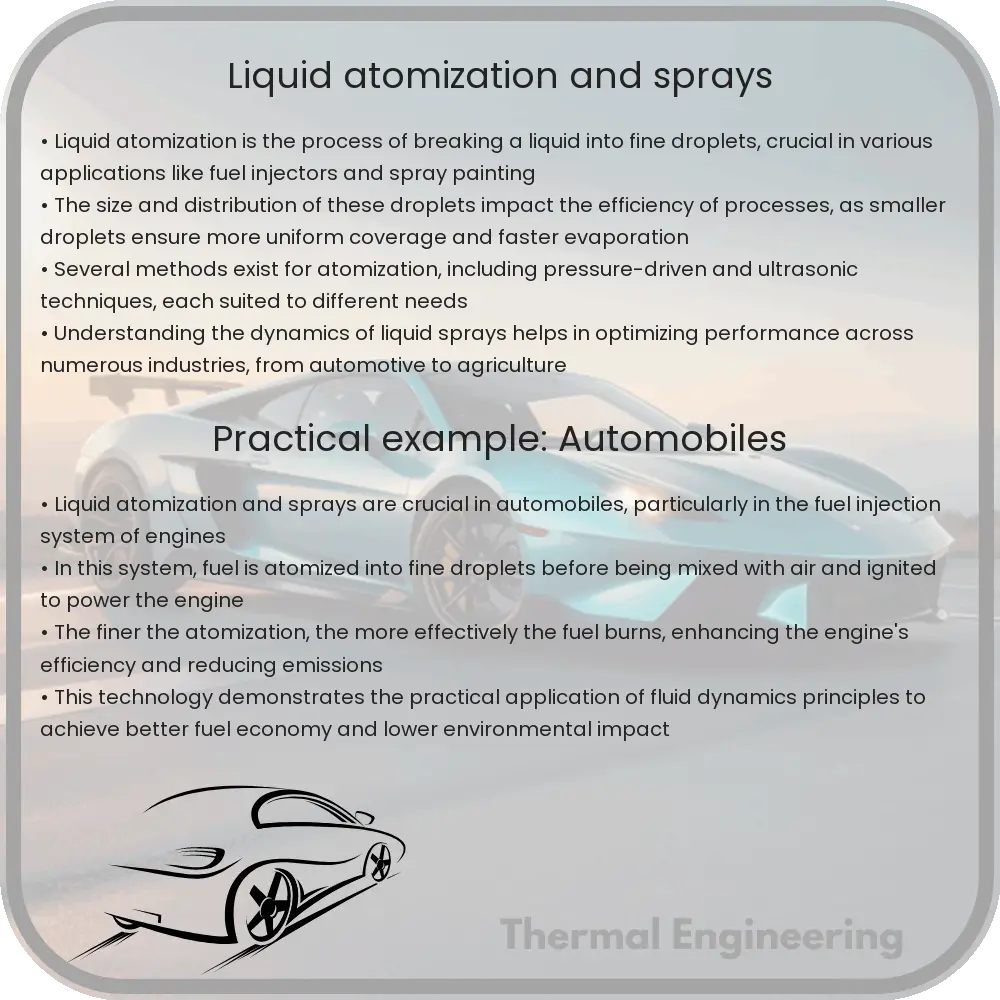
• Fuel Injection Systems: In automotive and aerospace engineering, atomization facilitates the fine and uniform spray of fuel, improving fuel-air mixing and combustion efficiency.
• Agricultural Sprays: Atomization ensures the even distribution of pesticides and fertilizers over crops, minimizing waste and environmental impact.
• Medical Nebulizers: In medical devices such as nebulizers, atomization is used to convert liquid medication into fine mists, which can be easily inhaled deep into the lungs.

Understanding and harnessing the principles of liquid atomization and sprays continues to be a vital area of research and development, leading to advances in technology, efficiency, and environmental protection.

Fire and smoke propagation involve complex interactions of heat, air flows, and chemical reactions, all of which can be studied through the principles of fluid mechanics. This field of engineering helps us understand how fire spreads in different environments and conditions, aiding in effective firefighting strategies and building safer structures.

Understanding the Fluid Mechanics of Fire and Smoke Propagation

Fire and smoke propagation involve complex interactions of heat, air flows, and chemical reactions, all of which can be studied through the principles of fluid mechanics. This field of engineering helps us understand how fire spreads in different environments and conditions, aiding in effective firefighting strategies and building safer structures.

Basics of Fluid Mechanics in Fire Dynamics

Fluid mechanics is a branch of physics concerned with the behavior of fluids (liquids and gases) in motion. It provides essential insights into how air movements affect fire behavior, including the spread of smoke. Two fundamental aspects of fluid mechanics in fire are buoyancy-driven flow and turbulent diffusion.

• Buoyancy-Driven Flow: Hot gases produced by fire are less dense than the cooler air surrounding them, creating an upward movement known as buoyancy. This can cause a fire to spread vertically through structures, commonly seen in scenarios like chimney effects in buildings.
• Turbulent Diffusion: The irregular, chaotic motion of gases contributes to the rapid spread of fire and smoke through increased mixing of hot gases and air. This turbulence enhances heat transfer and accelerates fire growth.

Mathematical Representation of Fire Dynamics

To predict and analyze fire and smoke behavior, engineers use mathematical models that describe the conservation of mass, momentum, and energy in fluid flows. The basic equations include:

1. Conservation of Mass (Continuity Equation): \( \frac{\partial \rho}{\partial t} + \nabla \cdot (\rho \vec{v}) = 0 \) where \( \rho \) is the fluid density and \( \vec{v} \) is the flow velocity vector.
2. Conservation of Momentum (Navier-Stokes Equations): \( \rho \left(\frac{\partial \vec{v}}{\partial t} + \vec{v} \cdot \nabla \vec{v}\right) = -\nabla p + \mu \nabla^2 \vec{v} + \vec{f} \) with \( p \) representing pressure, \( \mu \) the dynamic viscosity, and \( \vec{f} \) external forces like gravity.
3. Conservation of Energy: \( \frac{\partial}{\partial t}(\rho e) + \nabla \cdot (\rho e \vec{v}) = \nabla \cdot (k \nabla T) + \Phi \), where \( e \) is the internal energy per unit mass, \( T \) is temperature, \( k \) is thermal conductivity, and \( \Phi \) represents the dissipation function.

Applications in Safety Engineering

Understanding the fluid dynamics of fire and smoke is critical in designing safety measures for buildings and urban areas. This includes:

• Smoke Management Systems: Effective ventilation designs can help control smoke movement, maintaining clear evacuation routes during a fire.
• Building Layout Optimization: By studying how fire and smoke propagate, engineers can design building layouts that minimize fire spread and enhance containment.
• Fire Suppression Systems: Knowledge of fluid mechanics aids in the design of more efficient sprinkler systems that can effectively target hot spots and suppress fires quickly.

Challenges and Future Directions

Despite significant advances, predicting the precise behavior of fire and smoke remains a challenge due to the chaotic nature of turbulence and the complex chemical reactions involved in combustion. Future research aims to enhance computational models and incorporate new materials and building technologies to better understand and control fire dynamics.

In conclusion, the study of fluid mechanics provides essential insights into the unpredictable and dynamic nature of fire and smoke. By continuing to integrate advanced modeling techniques and interdisciplinary research, we can improve fire safety protocols and reduce the destructive impact of fires on society.

Learn about the causes and reduction techniques for fluid-induced noise in engineering systems like HVAC and automotive exhausts.

Understanding Fluid-Induced Noise and Its Reduction Techniques

Fluid-induced noise is a common issue in various engineering systems where fluids are in motion, such as in HVAC systems, pipelines, and automotive exhausts. This type of noise can not only be a nuisance but can also indicate inefficiencies or problems in system operation. Addressing fluid-induced noise effectively requires an understanding of its origins and implementing strategic reduction techniques.

Causes of Fluid-Induced Noise

Fluid-induced noise usually arises from several sources, primarily turbulence and interactions with solid boundaries. When a fluid flows at high velocity or through a constricted path, turbulence is generated. This turbulence can lead to fluctuations in pressure and velocity, which manifest as sound waves. Additionally, when these turbulent flows interact with surfaces or obstacles, further noise can be emitted due to vibration and secondary turbulent eddies.

Basic Approaches to Reduce Fluid-Induced Noise

1. Minimizing Turbulence: One of the primary methods to reduce noise is to control the flow turbulence. This can be achieved by designing smoother conduits and using flow straighteners or diffusers to stabilize the flow.
2. Vibration Damping: Since interactions between the fluid and system boundaries can generate noise, incorporating materials that damp vibrations can be effective. This includes the use of rubber mounts, insulation materials, or specialized composites that absorb vibrational energy.
3. Acoustic Insulation: Encapsulating noisy components with acoustic barriers or using materials with high sound absorption coefficients can significantly reduce noise emission into the surrounding environment.

Advanced Technologies for Noise Reduction

• Active Noise Control: This technique involves using an interference sound wave that is phase-inverted relative to the unwanted noise. When these two waves intersect, they can cancel each other out, reducing the overall noise level.
• Helmholtz Resonators: These are structures designed to capture and dissipate acoustic energy at specific frequencies. They are particularly effective for tuning out narrow-bandwidth noise emissions.
• Computational Fluid Dynamics (CFD): CFD can be utilized to simulate fluid flow and predict noise generation, helping in designing systems that minimize noise from the outset.

Practical Applications and Examples

In automotive engineering, effective exhaust silencers and engine covers are designed using principles of fluid dynamics and acoustics to reduce noise. In HVAC systems, duct designs often incorporate bends and expansion chambers that dissipate sound energy. Industry pipelines utilize varied diameter changes and padded clamps to reduce both vibration and noise transmission.

Conclusion

Fluid-induced noise not only affects comfort but also system efficiency and longevity. By understanding the mechanisms of noise generation and implementing both basic and advanced noise reduction techniques, engineers can create quieter and more efficient systems. Ongoing research and technological advancements continue to offer new solutions in combating fluid-induced noise, promising quieter environments and better performing machinery.

Magnetohydrodynamics (MHD) examines the dynamics of electrically conducting fluids in magnetic fields, impacting energy generation and management.

Understanding Magnetohydrodynamics in Energy Applications

Magnetohydrodynamics (MHD) may sound like a complex term, but it’s a fascinating field of study that combines the principles of both magnetism and fluid dynamics. The underlying concept involves the study of the dynamics of electrically conducting fluids like plasmas, liquid metals, and saltwater. The applications of MHD are wide-reaching but are particularly impactful in various energy systems. Let’s explore how MHD is used to enhance energy generation and management.

MHD Fundamentals

At its core, MHD deals with the behavior of fluids that can conduct electricity in the presence of a magnetic field. The interaction between the magnetic field and the electrically charged fluid generates forces that influence the fluid’s flow patterns. These dynamics are governed by a set of equations that combine Navier-Stokes equations of fluid dynamics and Maxwell’s equations of electromagnetism. Simplifying these complex interactions:

• Navier-Stokes Equation (Fluid Dynamics): Defines how the velocity field of fluid motion is affected by forces.
• Maxwell’s Equations (Electromagnetism): Describe how electric and magnetic fields are generated by charges, currents, and changes of the fields themselves.

The coupling of these equations produces the MHD equations, which describe the motion of the conducting fluid in the magnetic field.

Energy Generation through MHD

One of the most prominent applications of MHD is in the area of energy generation, specifically through MHD generators. These devices convert thermal energy and kinetic energy directly into electricity. The basic process involves a conductive fluid (often a hot, ionized gas called plasma) flowing through a magnetic field. The interaction between the fluid and the magnetic field induces an electromagnetic force according to Faraday’s Law of Electromagnetic Induction, typically expressed as:

E = -v * B

Where E is the induced electric field, v is the velocity of the fluid, and B is the magnetic field. This induced electric field can then be used to generate an electric current, which is harnessed as electrical power.

Benefits and Challenges

Using MHD in energy applications offers several advantages:

• Efficiency: MHD generators can convert energy directly from thermal to electrical forms, potentially bypassing the mechanical stages required in traditional power generation. This can result in higher efficiencies in energy conversion.
• Environmentally Friendly: MHD systems can operate at high temperatures and use clean fuels such as hydrogen, resulting in lower emissions of pollutants.

However, the challenges are significant:

• Materials: High temperatures and corrosive environments within MHD systems demand materials that can withstand extreme conditions without degrading.
• Cost: The initial setup and maintenance costs for MHD systems are currently high, limiting their widespread implementation.

Looking Ahead

Continuous research is being directed towards overcoming the challenges faced by MHD technology. Advances in materials science, improved magnet technology, and better understanding of fluid dynamics are paving the way for more efficient and economically viable MHD systems. Although still primarily in the experimental and developmental stage, the potential for MHD in sustainable energy systems continues to inspire scientists and engineers around the globe.

Magnetohydrodynamics represents an exciting intersection of physics and engineering with the potential to significantly impact how future energy systems are designed and implemented. For anyone interested in the future of energy, MHD offers a window into next-generation technology that balances efficiency with environmental consciousness.

Learn how thermal efficiency in gas turbines converts fuel heat into power, impacting performance and emissions.

Understanding the Thermal Efficiency of Gas Turbines

Gas turbines are widely used in various applications, ranging from aerospace engines to power generation. One of the critical aspects that determine the performance and environmental impact of gas turbines is their thermal efficiency. This measure indicates how well a turbine converts the heat energy from fuel into useful work or power. Improving thermal efficiency not only enhances performance but also reduces fuel consumption and emissions.

How Thermal Efficiency is Calculated

Thermal efficiency (\(\eta_{th}\)) of a gas turbine is typically calculated using the formula:

\[
\eta_{th} = \frac{Work output}{Heat input} \times 100\%
\]

This formula involves the ratio of the mechanical work output of the turbine to the total heat energy input from the fuel. The work output can further be expressed as the product of the turbine’s power output and time, whereas the heat input is the product of the fuel mass flow rate, the heating value of the fuel, and time.

Factors Affecting Thermal Efficiency

• Temperature: The efficiency of gas turbines significantly increases with the inlet temperature of the gas. Higher temperatures enable the turbine to extract more energy from the exhaust gases, though this is often limited by material strength and thermal characteristics of turbine components.
• Pressure Ratio: The ratio of the pressure at the turbine exit to the pressure at the turbine inlet also affects efficiency. Higher pressure ratios typically improve the efficiency but require more robust and sometimes more expensive materials to withstand the increased stress.
• Component Efficiency: The efficiencies of individual components of the turbine, such as the compressor and the combustor, also impact the overall thermal efficiency. Improvements in blade design, cooling methods, and combustion technology can lead to better component efficiency.

Technological Improvements

In the pursuit of higher thermal efficiencies, engineers and scientists focus on several technological advancements:

• Materials: Development of high-temperature materials like ceramic-matrix composites (CMCs) and superalloys that can withstand higher temperatures without degrading.
• Cooling Techniques: Advanced cooling methods for turbine blades, such as internal air channels and thermal barrier coatings, help in managing the heat loads while allowing higher operational temperatures.
• Combustion Technology: Innovations like lean-burn technology help in achieving more complete combustion of fuel, thereby increasing efficiency and reducing emissions.

The Role of Regeneration

One effective way to enhance the thermal efficiency of gas turbines is through regeneration. This process involves capturing some of the waste heat from the turbine exhaust and using it to preheat the compressed air entering the combustion chamber. By recovering this heat, the turbine requires less fuel to reach the desired temperature, thus improving efficiency.

Conclusion

Thermal efficiency is a key metric in the performance of gas turbines, influencing both operational costs and environmental sustainability. Through ongoing advancements in materials engineering, cooling technologies, and combustion processes, the efficiency of these powerful machines continues to improve, paving the way for more sustainable and economical power generation and aeronautical propulsion systems.

Hydraulic modeling of river systems involves simulating river behaviors and interactions for effective water management and environmental conservation.

Introduction to Hydraulic Modeling of River Systems

Hydraulic modeling of river systems is an essential branch of engineering that focuses on understanding and predicting the behavior of rivers and streams when subjected to various natural and anthropogenic factors. This technique employs mathematical and physical models to simulate water flow and associated processes within river networks. The primary goal is to aid in effective water resource management, flood protection, and environmental conservation.

The Basics of Hydraulic Modeling

The core of hydraulic modeling lies in its ability to represent the dynamic and often complex interactions between water flow and riverbeds. This includes the simulation of water currents, sediment transport, erosion, and deposition processes. Models can be broadly classified into two categories: physical models and mathematical (or numerical) models.

• Physical Models: These involve scaled-down constructions of river sections in controlled environments, where water flow and behavior can be studied physically.
• Mathematical Models: These are computer-based and use mathematical equations to simulate the physics of water flow. Commonly used mathematical models include the Saint-Venant equations for unsteady flow, which can be expressed as follows:

\[ \frac{\partial Q}{\partial t} + \frac{\partial (Q^2/A)}{\partial x} + gA\frac{\partial H}{\partial x} = gAS_f \]

Here, Q is the flow rate, A is the cross-sectional area of flow, H represents the depth of flow, t stands for time, x is the spatial coordinate, g denotes gravitational acceleration, and S_f is the friction slope.

Steps in Hydraulic Modeling

1. Data Collection: Gathering accurate field data is crucial for model calibration and validation. This includes hydrological data (like flow rates), meteorological data, and physical measurements of river geometries.
2. Model Selection and Setup: Choosing the appropriate model type (physical or mathematical) based on the specific requirements and goals of the project.
3. Calibration and Validation: Adjusting model parameters to match observed data and ensure the model accurately represents real-world conditions.
4. Simulation Runs: Performing model simulations under various scenarios to predict river behavior under different conditions, such as flood events, droughts, or anthropogenic changes like dam construction.
5. Analysis of Results: Analyzing simulation outputs to make informed decisions on water resource management, infrastructure development, and environmental protection.

Applications of Hydraulic Modeling

Hydraulic models are powerful tools in modern engineering and environmental management, providing valuable inputs for:

• Flood risk assessment and floodplain management
• Design and optimization of hydraulic structures like weirs, dams, and spillways
• Ecosystem restoration and habitat simulation studies
• Sediment management and control of riverbank erosion
• Disaster management and emergency response planning

Challenges and Future Directions

While hydraulic modeling provides numerous benefits, it faces challenges such as dealing with complex river topographies, varying hydraulic conditions, and the impacts of climate change on water resources. Advances in technology, including enhanced computational capacities, the integration of GIS (Geographic Information Systems), and real-time data acquisition, are continually improving the accuracy and efficiency of hydraulic models.

The future of hydraulic modeling lies in the convergence of more detailed environmental data, improved computational algorithms, and interdisciplinary approaches that blend engineering, geography, and ecological sciences to create more comprehensive and predictive tools for managing water resources and preserving river ecosystems.

Explore the dynamics of sediment transport in fluid flows, covering types, influencing factors, and mathematical models for real-world applications.

Understanding Sediment Transport in Fluid Flows

Sediment transport is a key phenomenon in both natural and engineered environments, affecting river landscapes, coastal areas, and infrastructure. This process involves the movement of solid particles, typically soil, sand, and gravel, carried by water, air, or ice. Fluid flows such as rivers, oceans, and wind play a crucial role in shaping the terrain by transporting these sediments from one location to another.

Types of Sediment Transport

There are three primary types of sediment transport that occur in fluid flows:

• Bedload Transport: This type involves particles that are rolled, slid, and hopped along the bottom of the riverbed or seabed. Bedload particles are typically larger and denser, requiring substantial energy to move.
• Suspended Load: Finer particles are carried within the fluid flow above the bottom surface. These sediments can be transported long distances by the flow due to their small size and lighter weight.
• Dissolved Load: This type refers to the chemical solution of minerals that are transported within the flow. Dissolved load is the result of water-rock interactions where minerals are chemically dissolved in water.

Factors Influencing Sediment Transport

Several factors affect how sediments are transported in fluid flows, which include:

• Fluid Velocity: The speed of the fluid plays a crucial role, with higher velocities able to transport larger and more sediments.
• Particle Size and Density: Larger and denser particles are generally harder to move and are typically transported as bedload.
• Viscosity of the Fluid: The internal friction of the fluid affects its capacity to carry sediments, with lower viscosity facilitating easier movement of particles.
• Slope of the Surface: Steeper slopes can increase the energy of the fluid flow, enhancing its ability to transport sediments.

Mathematical Models of Sediment Transport

To predict and analyze sediment transport, engineers and scientists use mathematical models that are based on the fundamental laws of physics, like conservation of mass and momentum. The Shield’s criterion, for example, is a dimensionless parameter used to determine whether particle movement will occur or not based on the force balance:

\( \tau^* = \frac{\tau}{(\rho_s – \rho) \cdot g \cdot d} \)

where:

• \( \tau^* \) (Shields parameter) is the dimensionless shear stress,
• \(\tau\) is the bed shear stress,
• \(\rho_s\) is the density of sediment particles,
• \(\rho\) is the fluid density,
• \(g\) is the acceleration due to gravity, and
• \(d\) is the diameter of sediment particles.

This formula helps assess whether the existing flow conditions can initiate particle motion, which is critical for understanding sediment dynamics in river engineering and coastal management.

Importance of Sediment Transport

The study of sediment transport is crucial for numerous practical applications, including:

• Flood risk management: Predicting sediment transport helps in designing flood defenses by understanding how rivers carry sediments during flood events.
• Coastal engineering: Coastal erosion and accretion are closely linked to sediment dynamics, important for beach nourishment projects and coastal structure design.
• Environmental restoration: Effective sediment management can help restore habitats affected by sediment depletion or excess.
• Waterway maintenance: Navigable channels and harbors require regular dredging which is based on sediment transport patterns.

Understanding sediment transport not only aids in addressing practical engineering problems but also enriches our knowledge of geological and ecological processes shaping our planet.

Explore the dynamics of turbulent flow over rough surfaces and its critical role in fluid mechanics and engineering applications.

Understanding Turbulent Flow over Rough Surfaces

Turbulent flow over rough surfaces is a fundamental concept in fluid dynamics, which has significant implications in various engineering fields, including aerospace, civil, and environmental engineering. Turbulence is the random, chaotic movement of fluid particles, as opposed to the orderly, layered flow known as laminar flow. The complexity increases when these flows interact with rough surfaces.

What is Turbulent Flow?

Turbulent flow occurs when the kinetic energy of a fluid exceeds the damping effect of its viscosity, leading to a chaotic state where eddies, swirls, and currents appear within the flow. This kind of flow typically happens at high velocities and in fluids with low viscosity. In contrast to laminar flow, which is characterized by smooth streamlines and predictability, turbulent flow is distinguished by mixing, irregularity, and diffusion.

Impact of Roughness on Turbulence

The roughness of a surface plays a crucial role in the transition from laminar to turbulent flow. Even minor imperfections on a surface can significantly alter the behavior of fluid flow. Rough surfaces increase the friction between the fluid and the surface, which enhances turbulence. These surfaces introduce additional eddies and disturbances in the flow, increasing the complexity of the fluid dynamics.

Quantifying Turbulence and Roughness

Two key dimensionless numbers help quantify the behavior of turbulent flows over rough surfaces:

• Reynolds Number (Re): This is a ratio of inertial forces to viscous forces in a fluid, given by the equation Re = (ρ * u * L) / μ, where ρ is the density of the fluid, u is the flow velocity, L is a characteristic linear dimension (like diameter of a pipe), and μ is the dynamic viscosity of the fluid. Higher Reynolds numbers indicate more turbulent flows.
• Roughness Ratio (k_s / L): This ratio represents the relative scale of the surface’s roughness (k_s) compared to the flow’s characteristic length scale (L). Higher values suggest more significant impacts of roughness on the flow.

Applications and Practical Considerations

Turbulent flow over rough surfaces is not just a theoretical concern but has practical implications in various engineering systems:

• Aerospace Engineering: Understanding the interactions between air flow and the rough surfaces of an aircraft can help optimize its performance and safety features.
• Civil Engineering: The design of hydraulic structures like dams, channels, and culverts relies on knowledge of how water interacts with rough surfaces to minimize erosion and energy loss.
• Environmental Engineering: Studying turbulent flow can aid in modeling pollution dispersion in rivers and atmospheric conditions.

Conclusion

The examination of turbulent flow over rough surfaces is essential for the accurate prediction and analysis of fluid behavior in various engineering applications. Understanding these dynamics allows engineers to design more efficient and effective systems, whether it be reducing drag on an aircraft, preventing erosion in water channels, or predicting environmental pollutant dispersal. This intersection of fluid mechanics and material science continues to challenge and advance the capabilities of modern engineering.

Explore the crucial role of fluid dynamics in chemical reactors, focusing on flow types, mixing, and reactor efficiency.

Understanding Fluid Dynamics in Chemical Reactors

Fluid dynamics plays a crucial role in the design and operation of chemical reactors, which are the heart of chemical engineering processes. The behavior of fluids affects mixing, reaction rates, heat transfer, and overall reactor efficiency. This article explores how fluid dynamics principles apply to chemical reactors and why understanding these principles is vital for optimal reactor design.

Basic Concepts of Fluid Dynamics in Reactors

Laminar and Turbulent Flow: Fluid flow within reactors can be categorized into two types: laminar and turbulent. Laminar flow, characterized by smooth and orderly fluid motion, is typically observed at low flow velocities and high viscosity conditions. In contrast, turbulent flow occurs at high velocities and involves chaotic changes in pressure and flow velocity. These flow regimes significantly affect the mixing and reaction rates in chemical processes.

Reynolds Number: The Reynolds number (Re) is a dimensionless quantity used to predict flow patterns in different fluid flow situations. It is defined as:

\[ Re = \frac{D * v * \rho}{\mu} \]

where D is the characteristic length (typically diameter), v is the fluid velocity, \rho is the density, and \mu is the viscosity of the fluid. A higher Reynolds number typically indicates turbulent flow, while a lower Reynolds number indicates laminar flow.

Role of Fluid Dynamics in Chemical Reaction Engineering

Mixing: Effective mixing is critical in chemical reactors to ensure uniform distribution of reactants and temperature. Fluid dynamics helps in designing impellers and baffles that enhance the mixing efficiency. In turbulent flow, mixing is generally more intense and rapid compared to laminar flow.

Heat Transfer: In exothermic and endothermic reactions, maintaining a controlled temperature within the reactor is vital to the safety and efficiency of the process. Fluid dynamics principles help in designing cooling and heating systems that maintain the optimal temperature by enhancing the convection process.

Mass Transfer: The rate of mass transfer, which is essential for the reaction to occur, is also influenced by the flow of fluids. In reactors, the design must promote efficient mass transfer to optimize reaction rates and yield.

Applications and Examples

• Stirred Tank Reactor: Often used in the chemical industry, these reactors use impellers to agitate the fluid, promoting homogeneous mixing and heat transfer. The design of the impeller and the tank geometry are influenced by fluid dynamic analysis to optimize performance.
• Fluidized Bed Reactor: These reactors allow for a high contact surface area between the reactant and catalyst by fluidizing solid catalyst particles using high-velocity fluid flow. Fluid dynamics helps in determining the optimal flow rate that ensures the fluidization without carrying the solid particles away.
• Packed Bed Reactor: Used for reactions involving gases and a solid catalyst, the fluid dynamics in packed beds focus on understanding how the fluid flows through the fixed bed of catalyst particles. This understanding is crucial to minimize pressure drops and maximize the reaction surface area.

Conclusion

Fluid dynamics is an essential aspect of designing and operating efficient chemical reactors. By understanding the flow characteristics and applying fluid dynamics principles, engineers can design reactors that improve mixing, maximize heat and mass transfer, and enhance the overall process efficiency. This leads to more cost-effective, safe, and environmentally friendly chemical processing industries.

Understanding and predicting ocean currents and their impacts on climate and ecosystems through ocean circulation modeling.

Ocean Circulation Modeling

Ocean circulation modeling is a critical branch of oceanography and environmental engineering, playing a key role in understanding and predicting the movements of ocean currents and their impacts on climate, ecosystems, and human activities. These models simulate the ocean’s fluid dynamics, heat transfer, and solute transport, contributing significantly to weather forecasting, climate change predictions, and disaster management.

Basics of Ocean Circulation

Ocean currents are primarily driven by two major forces: the wind and the thermohaline circulation, which is influenced by water density variations due to temperature (thermo) and salinity (haline) differences. Surface currents are largely wind-driven, whereas deeper water movements are mostly controlled by density gradients. Understanding these mechanisms is crucial for developing accurate ocean models.

Components of Ocean Circulation Models

• Hydrodynamic Modules: These modules simulate fluid motion using the Navier-Stokes equations, adapted for rotational and stratified flows typical of oceans.
• Thermodynamic Processes: They account for heat exchange between the ocean and atmosphere, including heating by solar radiation and cooling by evaporation.
• Salinity Transport: Models simulate the mixing and transport of various salts, crucial for maintaining the ocean’s density structure.
• Sea Ice Dynamics: Especially in polar models, the formation, movement, and melting of sea ice are integral components impacting overall ocean circulation.

Mathematical Foundations of Modeling

At the core of ocean circulation models are the primitive equations, which are a form of the Navier-Stokes equations simplified under the assumption of hydrostatic balance. The basic form of these equations can be expressed as:

1. The momentum equations in the x and y directions (horizontal):
   • dU/dt = -∂p/∂x + fv + other forces
   • dV/dt = -∂p/∂y – fu + other forces
2. The continuity equation (mass conservation):
   • ∂U/∂x + ∂V/∂y + ∂W/∂z = 0
3. The thermodynamic equation (heat equation):
   • dT/dt = -(U∂T/∂x + V∂T/∂y + W∂T/∂z) + heating/cooling

Here, U, V, and W represent the velocity components in the x, y, and z directions, respectively; p denotes pressure; T stands for temperature; and f is the Coriolis parameter, which accounts for the Earth’s rotation.

Challenges and Advances in Ocean Circulation Modeling

One of the most significant challenges in ocean circulation modeling is the vast scale and complexity of the oceans. High spatial resolution is required to accurately capture small-scale processes like eddies and turbulence, which are crucial for realistic simulations. Additionally, integrating data from disparate sources, such as satellite observations and in-situ measurements, remains a formidable task.

Recent advances in computational power and techniques, like data assimilation and machine learning, are progressively overcoming these challenges. Data assimilation involves combining model outputs with observational data to improve model accuracy, while machine learning algorithms are used to predict complex non-linear interactions within the ocean system.

Conclusion

Ocean circulation models are indispensable tools for marine and climate scientists. They provide valuable insights into both current state and future changes in oceanic and atmospheric conditions. As technology and methodologies continue to evolve, these models will become increasingly accurate and detailed, offering more reliable forecasts and a better understanding of our planet’s intricate climate system.