Thermal Engineering

Learn about fluid dynamics principles essential for flow measurement, vital in engineering disciplines like aerospace and chemical engineering.

Understanding Fluid Dynamics: Principles of Flow Measurement

Fluid dynamics, a sub-discipline of fluid mechanics, involves the study of fluids (liquids and gases) in motion. Understanding how fluids move and react in different environments is crucial for several engineering disciplines, including aerospace, civil, and chemical engineering. This article explores the fundamental principles of flow measurement, an essential aspect of fluid dynamics.

What is Flow Measurement?

Flow measurement refers to the quantification of bulk fluid movement. Engineers and scientists measure the flow rate to determine the amount of fluid passing through a particular point per unit time. Common units include liters per second (L/s), cubic meters per hour (m³/h), or gallons per minute (GPM).

Types of Flow

• Laminar Flow: This type of flow occurs when a fluid flows in parallel layers, with no disruption between the layers.
• Turbulent Flow: In turbulent flow, the fluid undergoes irregular fluctuations or mixing. It is characterized by rapid changes in pressure and velocity within the fluid.
• Transient Flow: This flow type involves time-dependent changes in the flow rate. The conditions of the flow change with time, such as when a pump is switched on or off.

Key Methods of Flow Measurement

Different techniques are applied to measure fluid flow, each suitable for specific types of fluids and flow conditions. Here are some of the most commonly used methods:

1. Volumetric Flow Meters: These devices measure the volume of fluid passing through a point over time. Examples include piston meters, gear meters, and oval gear meters.
2. Mass Flow Meters: Utilized extensively in chemical applications and industries, these meters measure the mass flow rate of a fluid traveling through a tube. Technologies include thermal mass flow meters and Coriolis flow meters.
3. Velocity Flow Meters: These measure the velocity of fluid and convert it into a flow rate. Common types include turbine, paddlewheel, and electromagnetic flow meters.
4. Differential Pressure Flow Meters: This method is one of the oldest and is based on changes in pressure drop across a flow constriction, which correlates to flow rate. Examples include orifice plates, flow nozzles, and venturi meters.

Equations and Concepts

In fluid dynamics, the basic equation used to calculate volumetric flow rate (Q) is:

Q = A * V

where:

• A is the cross-sectional area of the pipe (m²).
• V is the velocity of the fluid (m/s).

For mass flow rate (ṁ), the equation is:

ṁ = ρ * Q

where:

• ρ is the density of the fluid (kg/m³).

Understanding these principles and measurements is crucial for the design and operation of systems in various engineering fields. Correctly measuring flow is essential for ensuring operational efficiency, safety, and compliance with environmental standards.

Conclusion

The principles of flow measurement in fluid dynamics are vital for engineers across many disciplines. By accurately measuring and analyzing fluid flow, improvements can be continually made in the design and function of equipment and systems, leading to better performance, increased safety, and optimal use of resources.

Understanding these fundamentals allows engineers and scientists to solve complex problems in fluid mechanics, making it an integral part of engineering education and application.

Learn how the Venturi tube utilizes the Venturi effect to measure the flow rate of fluids in various engineering applications.

Understanding the Venturi Tube and Its Application in Measuring Flow Rate

The Venturi tube is a device used in various engineering fields to measure the flow rate of fluids flowing through a pipe. It is based on the Venturi effect, which is a fluid dynamics principle stating that fluid pressure decreases as the speed of the fluid increases.

Principle Behind the Venturi Tube

The Venturi tube was invented by Giovanni Battista Venturi, an 18th-century Italian physicist. The basic principle of the Venturi tube involves a constriction within the tube that causes a change in fluid speed and pressure. According to the principle of conservation of energy, specifically Bernoulli’s equation, the total energy in a steadily flowing fluid system is conserved. Bernoulli’s equation can be stated as:

E = (p + ½ρv² + ρgh) = constant

• p is the fluid pressure
• ρ (rho) is the fluid density
• v is the fluid velocity
• g is the acceleration due to gravity
• h is the height above a reference level

In the case of horizontal flow where height change is negligible, the equation simplifies to:

p₁ + ½ρv₁² = p₂ + ½ρv₂²

Here, ₁ and ₂ denote conditions at two different points along the tube, before and after the constriction respectively.

How Venturi Tubes Measure Flow Rate

The operation of a Venturi tube in measuring flow rate involves the following steps:

1. A fluid flows through a pipe with a Venturi tube, which has a constricted section (the throat).
2. The flow speed increases as the fluid enters the throat due to the reduced cross-sectional area.
3. According to Bernoulli’s principle, the increase in fluid speed at the throat leads to a decrease in pressure.
4. Pressure sensors are placed before the constriction and at the throat. The difference in pressure (Δp = p₁ – p₂) is measured.
5. The flow rate (Q) of the fluid can then be calculated using the continuity equation and the measured pressure difference. The equation used is:

Q = A₂ * (sqrt((2 * Δp * ρ) / (ρ * (1 – (A₂ / A₁)²))))

• A₁ and A₂ are the cross-sectional areas of the pipe before and at the constriction, respectively.
• sqrt denotes the square root function.

Applications of Venturi Tubes

Venturi tubes are used widely across many industries due to their simplicity and reliability. Some of their applications include:

• Measurement of liquid flow in chemical and process industries.
• Air flow measurement in HVAC systems.
• Water flow measurement in irrigation and water management systems.

By providing a simple yet efficient method to measure flow rate without moving parts, Venturi tubes play a crucial role in many engineering systems where knowing the precise flow of fluids is essential.

Learn about surface tension, a crucial fluid property impacting engineering, technology, and nature.

Understanding Surface Tension in Fluids

Surface tension is a fundamental concept in the field of fluid mechanics, which plays a critical role in various engineering and natural processes. From the way water beads up on a waxed car hood to the operation of tiny micropumps in medical devices, understanding surface tension helps engineers and scientists manipulate and utilize fluids in innovative ways.

What is Surface Tension?

Surface tension is a property of the surface of a liquid that allows it to resist an external force, due to the cohesive nature of its molecules. The top layer of molecules in a liquid are not surrounded by similar molecules on all sides, and thus they cohere more strongly to those directly associated with them on the surface. This forms a film of molecules that makes the surface act like a stretched elastic membrane.

Causes of Surface Tension

The primary cause of surface tension is the cohesive forces between liquid molecules. These are typically due to hydrogen bonds in water or van der Waals forces in other liquids. The energy responsible for the formation of surface tension acts to minimize the surface area of a liquid, a principle that has profound implications in the behavior of fluids.

Mathematical Representation of Surface Tension

Surface tension (γ) can be quantitatively defined as the force along the surface of a liquid that acts at a right angle to any line segment in contact with the air. It is typically measured in Newtons per meter (N/m). Mathematically, it is expressed as:

\[ \gamma = \frac{F}{L} \]

where F is the force in Newtons and L is the length in meters over which the force acts.

Applications of Surface Tension

• Capillary Action: This is the ability of a liquid to flow in narrow spaces without the assistance of external forces (like gravity). It is a result of surface tension and is critical in various applications including the movement of water in plants and the operation of thin paper inkjet printer nozzles.
• Detergents and Soaps: These reduce the surface tension of water making it easier to spread and mix with oil and grease, enhancing cleaning efficiency.
• Medical Applications: In pulmonary medicine, surface tension is relevant for the functionality of the human lung. Surfactants in the lung reduce the surface tension, aiding in the lung’s ability to expand and contract.
• Inkjet Printing: Inkjet printers utilize surface tension to drop precise amounts of ink onto paper. Engineers design ink with specific surface tension properties to ensure it does not smear or bleed excessively.

Challenges and Future Prospects

The manipulation of surface tension is critical in the development of advanced materials and technologies. Engineers constantly research ways to alter surface tension through chemical means or by altering the physical environment to improve industrial processes. Future prospects include the development of more efficient drug delivery systems and enhanced oil recovery methods that manipulate surface tension at the molecular level.

In conclusion, surface tension is more than just a curious property of fluids; it is a pervasive effect that influences many technologies and natural phenomena. Understanding and controlling surface tension is a key component in a wide range of engineering disciplines and continues to be a vibrant area of research and applied science.

Learn about fire tube boilers, their construction, operation, and applications in heating and industrial processes.

Understanding the Fire Tube Boiler

Fire tube boilers are a type of boiler which has been in use since the early 19th century. They are designed to heat water by channeling combustion gases through tubes that run through a sealed container of water. This setup is one of the earliest forms of boiler systems, making it a fundamental piece of engineering in the industrial revolution and continuing to serve varied applications today.

Basic Construction and Operation

Fire tube boilers consist of a cylindrical shell sealed at both ends with the tubes running through it. The boiler’s main components include the shell, burner, fire tubes, smokestack, and sometimes also controls and safety devices. Fundamentally, the boiler operates by using fuel (commonly oil, gas, or coal) to heat water through the energy released by combustion gases.

• Shell: This is the outermost part, holding the water to be heated.
• Fire Tubes: These tubes run through the shell and act as the conduit through which hot gases pass. The heat from these gases is transferred to the water around the tubes.
• Burner: Located at one end of the boiler, it’s responsible for starting the combustion process.
• Smokestack: Also known as a chimney, it allows the exhaust gases to escape into the atmosphere.

Working Principle

In a fire tube boiler, the burner generates hot gases which are then circulated through the tubes embedded within the water. The heat from these gases is conducted through the walls of the tubes and transferred to the water. Consequently, the water heats up and eventually produces steam.

The process involves three main steps:

1. Heat Transfer: The hot gases generated from the burner pass through the fire tubes. The heat is transferred from the gases through the tube walls via thermal conduction, heating the water surrounding the tubes.
2. Steam Production: As water in the outer shell heats up, it begins to boil and transform into steam. The creation of steam in a closed vessel increases the pressure inside the boiler.
3. Steam Utilization: This high-pressure steam is then channeled through pipes for various industrial applications, including running turbines for electricity or for heating purposes in buildings.

Advantages and Applications

Fire tube boilers offer several advantages. They are simpler in design compared to water tube boilers and generally have lower initial costs. These boilers are compact in structure and have a high steam storage capacity. Due to their robust design and ease of operation, they require less stringent water quality control, making them favorable for regions with hard water.

Traditionally, fire tube boilers have been employed in steam locomotives, heating systems for residential and commercial buildings, and various smaller industrial facilities. Although less efficient in handling high pressure compared to water tube boilers, their simplicity makes them still popular in less demanding applications.

In conclusion, the fire tube boiler represents a fundamental engineering advancement that continues to be an essential component of modern heating processes in various industries. Its simple design and function make it a reliable choice for many heating applications.

Learn about cooling curves, a key tool in thermal analysis for understanding material properties as they cool, used in materials science and engineering.

Understanding the Cooling Curve in Thermal Analysis

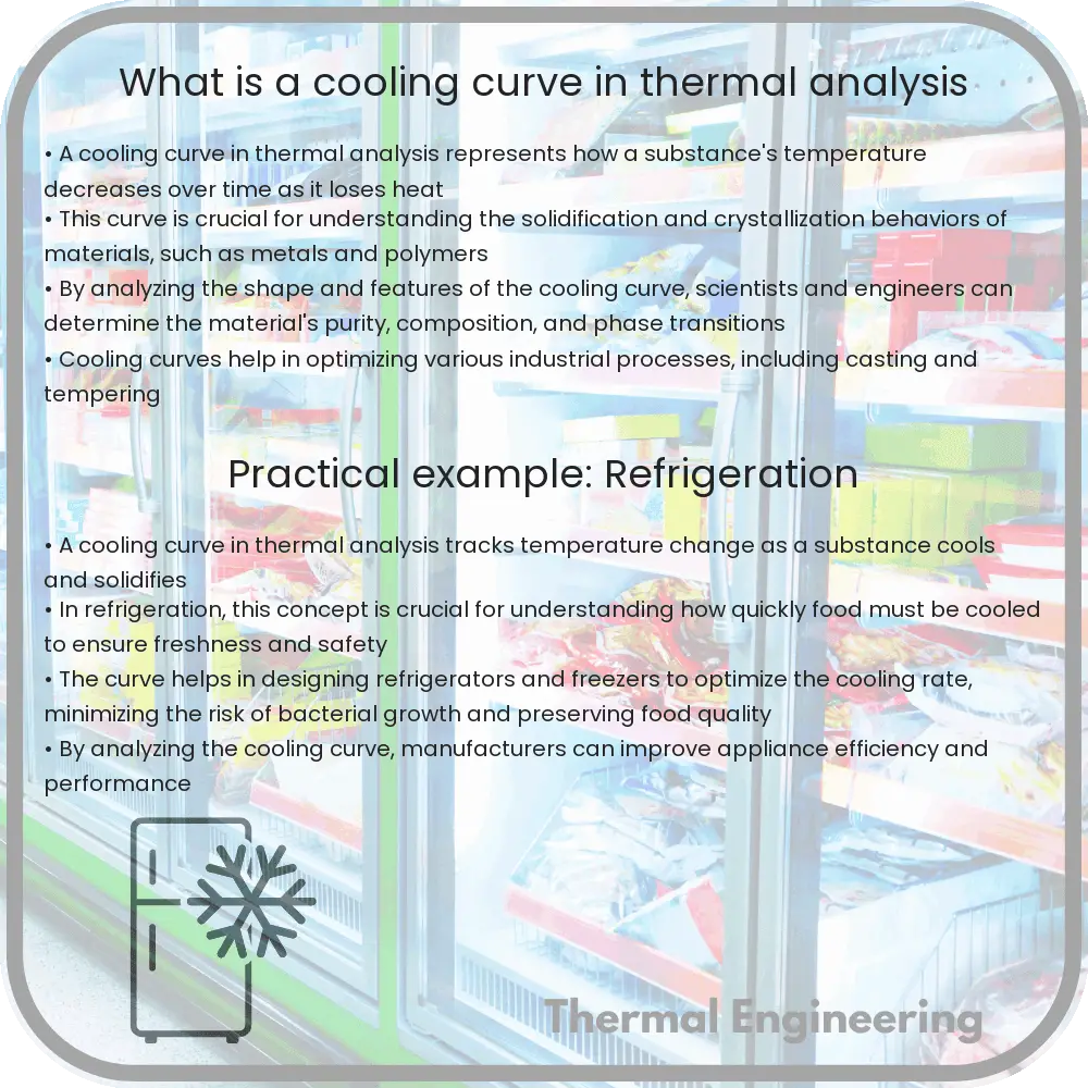
In the world of materials science and engineering, understanding how substances change with temperature is crucial. A cooling curve is a simple yet informative tool used in thermal analysis to study the transformations that occur as a material cools down from a high temperature, typically after having been melted.

What is a Cooling Curve?

A cooling curve graphically represents the change in temperature of a substance over time as it loses heat. This curve is typically plotted with temperature on the y-axis and time on the x-axis. The shape of the curve provides significant insights into the physical properties of the material, including its melting or freezing points, thermal conductivity, and latent heat.

How Is a Cooling Curve Generated?

To generate a cooling curve, a substance is initially heated to a temperature above its melting point, ensuring it transforms into a liquid. As the substance begins to cool, its temperature is meticulously recorded at regular intervals. Various phenomena observed during cooling, such as phase changes, significantly affect the heat release rate and consequently the shape of the cooling curve.

Key Segments of the Cooling Curve

• Liquid Region: This portion represents the time during which the material remains entirely in the liquid phase. The cooling rate might be relatively steady here, indicative of the substance’s specific heat capacity in liquid form.
• Phase Transition Plateau: As the substance begins to solidify, the temperature temporarily stabilizes. This plateau indicates a phase change, typically from liquid to solid. During this phase, the substance releases latent heat, which counters the cooling process, thus maintaining a relatively constant temperature.
• Solid Region: Once the entire material solidifies, the cooling curve resumes its downward trajectory. The slope in the solid region can provide information about the thermal conductivity and specific heat capacity of the solid material.

Practical Applications of Cooling Curves

Cooling curves are extensively used in metallurgy to determine the properties of metals and alloys. By analyzing where the phase transition plateaus occur, scientists and engineers can deduce the melting points of various components of an alloy. Furthermore, cooling curves can help in identifying impurities and predicting the mechanical properties of the material based on how it cools.

Conclusion

The cooling curve is a foundational tool in thermal analysis used to investigate the thermal properties of materials during the cooling phase. Its simplicity in setup and wealth of information make it invaluable in materials engineering, providing crucial insights into the physical characteristics of metals, alloys, and other materials. By studying how substances behave at different temperatures, engineers can enhance material design and functionality for a vast range of applications.

Learn about low thermal conductivity materials, their unique properties, applications across industries, and their role in enhancing energy efficiency.

Understanding Low Thermal Conductivity Materials

Low thermal conductivity materials are essential in various engineering applications where minimizing heat transfer is crucial. These materials, known for their ability to provide insulation, play a crucial role in industries ranging from building construction to aerospace. In this article, we explore what makes these materials unique, how they are utilized, and the types of materials typically used.

Basics of Thermal Conductivity

Thermal conductivity is a physical property that measures a material’s ability to conduct heat. It is denoted by the symbol ‘k’ and typically expressed in units of Watts per meter-Kelvin (W/m·K). The formula to calculate the rate of heat transfer (Q) through a material is given by Fourier’s law of heat conduction:

Q = -k * A * (dT/dx)

• A represents the area through which the heat is transferred,
• dT/dx is the temperature gradient across the material.

Materials with low thermal conductivity have a lower ‘k’ value, making them effective as insulators since they slow down the transfer of heat.

Characteristics of Low Thermal Conductivity Materials

Materials with low thermal conductivity share several common characteristics:

• Poor Thermal Conductors: These materials do not conduct heat efficiently, which makes them ideal for applications where heat retention or isolation is desired.
• High Thermal Resistance: They provide high resistance against heat flow, which enhances energy efficiency in thermal management systems.
• Low Density and Porosity: Many low thermal conductivity materials are lightweight and may have a porous structure, which contributes to their insulating properties.

Applications of Low Thermal Conductivity Materials

Low thermal conductivity materials are used in a wide range of applications, including:

• Building Insulation: These materials are commonly used in the walls, roofs, and foundations of buildings to prevent heat transfer, thereby maintaining a comfortable indoor environment while reducing energy costs.
• Thermal Barriers in Engines: In automotive and aerospace engineering, these materials are applied as thermal barrier coatings on engine parts to prevent overheating and improve efficiency.
• Cryogenics: Low thermal conductivity is critical in cryogenics for storing and handling very low temperature substances without significant heat gain.

Common Low Thermal Conductivity Materials

Several materials are known for their low thermal conductivity:

• Fiberglass: Widely used in building insulation, fiberglass consists of fine glass fibers and exhibits thermal conductivity values around 0.04 W/m·K.
• Polystyrene: A synthetic aromatic polymer made from the monomer styrene, polystyrene is another popular insulator in packaging and construction, with thermal conductivity around 0.033 W/m·K.
• Aerogels: Known as the lightest solid materials, aerogels have extremely low thermal conductivity (as low as 0.015 W/m·K) and are used in highly specialized environments like aerospace.

Future Outlook

The demand for efficient thermal insulation continues to drive innovation in the development of materials with even lower thermal conductivities. Research is ongoing in areas such as nanotechnology and composite materials, focusing on enhancing the insulating properties of materials while maintaining other necessary structural and functional characteristics. As technology advances, the role of low thermal conductivity materials is set to expand in existing markets and new innovative applications.

Understanding the properties and applications of low thermal conductivity materials not only enhances our ability to manage heat in industrial and daily contexts but also contributes to global energy efficiency goals, highlighting the importance of continued research and development in this area.

Learn about Phase Change Materials (PCMs), substances crucial for energy storage and regulation by leveraging latent heat during state transitions.

Understanding Phase Change Materials

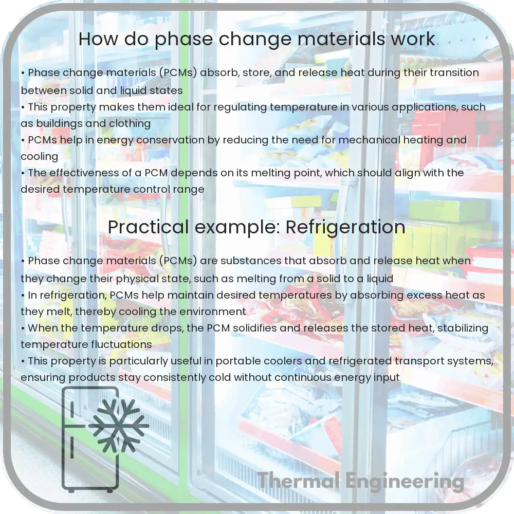
Phase Change Materials (PCMs) are substances that absorb and release thermal energy during the process of melting and freezing. They play a pivotal role in various applications ranging from building heating and cooling systems to renewable energy storage. PCMs operate on the simple principle of energy exchange through phase transition—primarily between solid and liquid states.

How Phase Change Materials Work

At the core of a PCM’s function is the latent heat of fusion—the energy absorbed or released during a change in state, with no change in temperature. When a PCM absorbs heat from its surroundings, it changes from a solid to a liquid, effectively storing this thermal energy in the form of latent heat. Conversely, when the environment cools, the PCM releases the stored heat as it returns to its solid state.

Key Types of Phase Change Materials

• Organic PCMs: These include materials like paraffin waxes and fatty acids. They are notable for their congruent melting, chemical stability, and minimal supercooling.
• Inorganic PCMs: Examples are salt hydrates and metallics which are characterized by higher latent heat per unit volume than organics but can suffer from phase separation and corrosion.
• Bio-based PCMs: These are extracted from agricultural resources and are both biodegradable and non-toxic, offering an environmentally friendly option.

Applications of Phase Change Materials

PCMs are utilized in a range of sectors to enhance efficiency and effectiveness in energy use:

1. Thermal Energy Storage: In solar energy systems, PCMs store excess heat collected during peak sunshine hours, which is then used to heat homes or commercial buildings during the night or on cloudy days.
2. Building Temperature Regulation: Incorporating PCMs in building materials, such as walls and floors, helps maintain a stable indoor environment, reducing the need for air conditioning and heating.
3. Temperature Controlled Transport: PCMs are used in packaging for temperature-sensitive goods, such as pharmaceuticals and perishable foods, ensuring they maintain quality during transit.

Challenges and Future Opportunities

While PCMs offer notable advantages, they are not without their challenges. Key issues include cost-effectiveness, long-term reliability, and integration with existing systems. Future advancements are likely to focus on improving PCM composites for greater stability, expanding the range of temperatures in which they can effectively operate, and enhancing their overall sustainability.

In conclusion, Phase Change Materials present a fascinating and potent tool in the quest for efficient energy management. By harnessing the properties of these materials, scientists and engineers can significantly impact how thermal energy is utilized across various industries, potentially leading to more sustainable practices and innovations in temperature regulation technology.

Learn about the Rankine cycle, a key thermal engineering concept crucial for converting heat into electricity in power plants.

Understanding the Rankine Cycle in Thermal Engineering

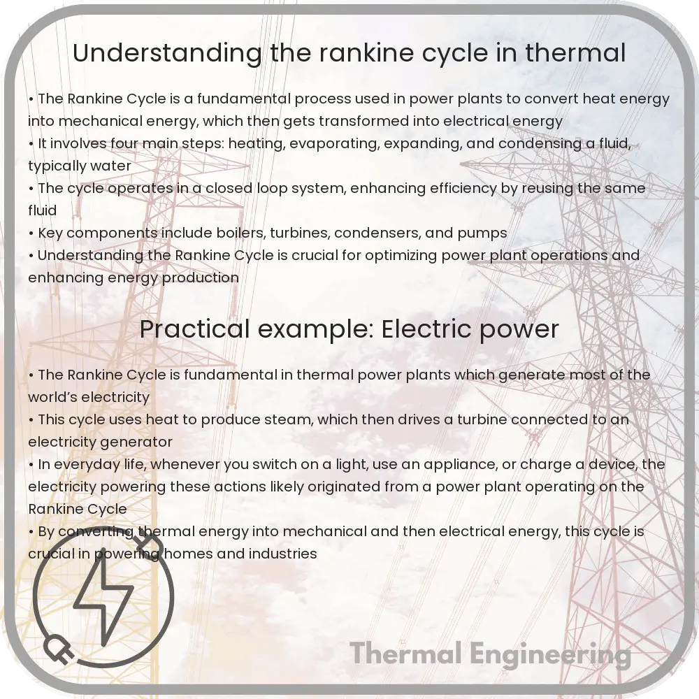
The Rankine cycle is a fundamental concept in thermal engineering and is the basic operation cycle of all thermal power plants. This process is used to convert heat into mechanical energy, which then can be transformed into electricity. In this article, we will explore the basic components and principles of the Rankine cycle.

Components of the Rankine Cycle

The Rankine cycle consists of four main components: a boiler, a turbine, a condenser, and a feed pump. Together, these components leverage the properties of water and steam to produce work. Here is how each part contributes to the cycle:

• Boiler: This is where liquid water is converted into steam using heat energy from various sources like coal, natural gas, or nuclear reactors.
• Turbine: The high-pressure steam generated in the boiler expands in the turbine, producing mechanical work that can drive an electricity generator.
• Condenser: After leaving the turbine, the steam is cooled back into liquid water by releasing heat into the surroundings.
• Feed Pump: This component increases the pressure of the condensed fluid, feeding it back into the boiler, thus completing the cycle.

The Thermodynamic Process of the Rankine Cycle

The Rankine cycle operates on a closed loop and can be broken down into four key thermodynamic processes:

1. Process 1-2 (Isentropic compression): Water at low pressure is pumped to a high pressure in the feed pump, raising its temperature slightly due to compression.
2. Process 2-3 (Constant pressure heat addition): High-pressure water enters the boiler, where it is heated and converted to steam at constant pressure.
3. Process 3-4 (Isentropic expansion): The high-temperature steam expands in the turbine, lowering its temperature and pressure, and in the process, mechanical work is done by the turbine.
4. Process 4-1 (Constant pressure heat rejection): The low-pressure steam is then condensed in the condenser at a constant pressure, releasing the heat to the surroundings and turning back into liquid water.

Each of these steps corresponds to physical changes within the water and steam, governed by laws of thermodynamics such as the conservation of energy and the increase of entropy.

Efficiency of the Rankine Cycle

The efficiency of a Rankine cycle is highly dependent on the temperatures and pressures of the steam. Higher efficiencies can be achieved by raising the steam’s temperature and pressure at the turbine’s inlet. However, practical limits are set by the material properties of the turbine and boiler, which can only withstand certain maximum temperatures and pressures.

Modifications to Improve Rankine Cycle Performance

Various modifications can be introduced to the classic Rankine cycle to enhance its efficiency and adapt it to different working conditions:

• Reheat Rankine Cycle: Steam is reheated after partial expansion to regain its energy, allowing for a double expansion in the turbine, incrementally improving the cycle’s efficiency.
• Regenerative Rankine Cycle: Heat exchangers are used to preheat the feed water entering the boiler using the steam extracted from different stages of the turbine. This saves fuel and increases overall efficiency by reusing the heat.

In summary, the Rankine cycle forms the backbone of modern thermal power generation systems. Understanding its basic principles and components provides a critical foundation in thermal engineering, helping to drive innovations and efficiency improvements in power generation.

Explore how heat pumps provide energy-efficient heating and cooling by leveraging thermodynamic principles, ensuring optimal performance across various climates.

Understanding the Principles of Heat Pump Efficiency

Heat pumps are increasingly popular devices that provide an energy-efficient alternative to furnaces and air conditioners. They work by moving heat rather than generating it, allowing them to heat and cool spaces with significantly reduced energy consumption. To truly appreciate the utility of heat pumps, it is essential to understand the principles that govern their efficiency.

How Heat Pumps Work

At their core, heat pumps operate based on the principles of thermodynamics, utilizing the heat transfer by absorbing heat from a cooler space and releasing it into a warmer one. This process involves four main components: the evaporator, the condenser, the compressor, and the expansion valve. The cycle starts in the evaporator, where the refrigerant absorbs heat and evaporates; the compressor then pressurizes the vapor, increasing its temperature. This hot vapor moves through the condenser, releasing the absorbed heat into the heating system before the refrigerant returns to liquid form and the cycle repeats.

Measuring Heat Pump Efficiency

The efficiency of heat pumps is most commonly measured by the coefficient of performance (COP) and the Seasonal Energy Efficiency Ratio (SEER). The COP measures the ratio of heat output to electrical energy input. It is generally higher in conditions where the temperature differential between the heat source and destination is smaller.

• The equation for COP is given by:
  
  COP = Heat Output (W) / Electrical Input (W)

The SEER, on the other hand, measures the cooling efficiency of the heat pump over a typical cooling season. It is calculated by the ratio of the cooling output across the season to the total electrical energy input during the same period.

• The formula for SEER is similar to COP but over an extended period:
  
  SEER = Total Cooling Output (Wh) / Total Electrical Energy Input (Wh)

Factors Affecting Heat Pump Efficiency

Several factors can influence the efficiency of heat pumps, including the external temperature, the quality of installation, and maintenance. Here’s how these factors play out:

1. External Temperature: Heat pumps are most efficient in mild climates. When the temperature drops too low, the COP decreases and additional energy may be required to maintain efficiency.
2. Installation Quality: Proper installation is essential for optimal heat pump performance. Incorrect sizing or poor handling can lead to inefficient operation and higher energy costs.
3. Maintenance: Regular maintenance such as checking filters, ducts, and refrigerant levels ensures that the heat pump operates at peak efficiency.

Advancements in Heat Pump Technology

Recent advancements in heat pump technology focus on improving efficiency even in colder climates. Innovations like dual-source heat pumps, which combine the features of air-source and geothermal heat pumps, and variable-speed compressors that adjust their output to the current demand, are making it possible to reap the benefits of heat pumps in a wider range of temperatures and settings.

In conclusion, understanding the efficiency of heat pumps is crucial when considering them as a potential heating and cooling solution. By measuring their performance through COP and SEER, and taking factors like climate, installation, and maintenance into account, one can maximize the benefits afforded by this sophisticated yet environmentally friendly technology.

Learn how the Mollier Diagram visually represents steam properties like pressure, temperature, and enthalpy for engineering applications.

Understanding the Mollier Diagram for Steam

The Mollier Diagram, named after Richard Mollier who first introduced it in 1904, is a graphical representation of the physical properties of moist air. It is an essential tool used in engineering, particularly in the fields of thermodynamics and HVAC (heating, ventilation, and air conditioning) systems. The diagram provides a visual representation of how different properties of steam, such as pressure, temperature, enthalpy, entropy, and volume, interrelate. This can be especially useful in designing and analyzing the performance of steam turbines, boilers, and other equipment where steam is used as a working fluid.

Understanding the Axes

The Mollier Diagram is usually plotted with entropy (s) on the x-axis and enthalpy (h) on the y-axis. Enthalpy represents the total heat content of the steam, while entropy is a measure of the steam’s disorder or randomness. Each line on the diagram represents a series of constant values for different properties:

• Temperature lines: These are almost vertical lines that slant slightly to the left, indicating the temperature of the steam at various combinations of entropy and enthalpy.
• Pressure lines: These lines are also nearly vertical but slant slightly more than temperature lines. They represent the pressure of the steam.
• Specific volume lines: Represented by lines that are horizontally oriented, showing the space occupied by a specific mass of steam.
• Saturation curve: This is a distinct curve that separates the diagram into two regions – the left of the curve denotes the wet region (where steam contains moisture), and the right side denotes the superheated steam region.

Reading the Diagram

To effectively use a Mollier Diagram, you need to be able to find a specific point on the diagram, which corresponds to the state of steam at any given condition. From this point, you can read off various properties directly:

• Finding a known property: For example, if the pressure and temperature of steam are known, locate the pressure line first, then move along this line to the point where it intersects with the corresponding temperature line.
• Reading other properties: From this intersection point, you can read directly or follow lines to find other properties such as specific volume, enthalpy, or entropy.

Applications of Mollier Diagram

The Mollier Diagram is extensively used in engineering analysis and design involving steam. Some common applications include:

• Steam turbine design and analysis: Engineers use the diagram to estimate the work output and efficiency of different stages of the turbine.
• Heat exchangers: The diagram can be used to analyze the heat transfer between steam and other mediums without direct interaction.
• Refrigeration cycles: Though primarily for steam, similar diagrams can be used for refrigerants in various refrigeration cycles to analyze and optimize performance.

Conclusion

The Mollier Diagram for steam is a vital graphic representation that aids in the understanding and calculation of the thermodynamic properties of steam. By allowing engineers to visualize the relationships and interactions between different properties of steam, it greatly simplifies the process of designing and optimizing thermal systems. Whether for educational or professional purposes, mastering the Mollier Diagram is essential for anyone involved in thermodynamics and HVAC system design and analysis.