Thermal Engineering

Exploring the benefits and applications of liquid metal cooling in engineering for enhanced thermal management in high-heat environments.

Liquid Metal Cooling in Engineering

Liquid metal cooling represents a cutting-edge approach in thermal management systems, particularly in fields where efficient heat dissipation is crucial. This method leverages the superior thermal conductivity and low viscosity of liquid metals to achieve highly effective cooling across various applications.

Principles of Liquid Metal Cooling

Liquid metals, such as gallium, indium, or their alloys, exhibit excellent thermal conductivity—surpassing that of conventional coolants like water or oil. Gallium-based alloys, for example, have a thermal conductivity around 40 W/m*K, significantly higher than water’s 0.6 W/m*K. This high thermal conductivity, combined with a low viscosity, enables efficient heat transfer.

The basic principle behind liquid metal cooling is simple: liquid metal absorbs heat from the object being cooled and is then circulated away to a heat exchanger, where the absorbed heat is released. The cooled liquid metal is then recycled back into the system.

Applications of Liquid Metal Cooling

• High-Performance Computing (HPC): As the demand for faster computational speeds and miniaturization continues, traditional cooling methods become less effective. Liquid metal cooling can handle the higher heat flux generated by compact and powerful HPC systems more efficiently.
• Electric Vehicles (EVs): In EVs, efficient thermal management is essential for battery longevity and performance. Liquid metal cooling systems can effectively manage the heat produced by EV batteries and electronic components.
• Nuclear Reactors: Advanced nuclear reactors utilize liquid metal cooling to manage the extreme heat generated during fission processes. This method enhances safety by facilitating more efficient heat removal and reducing the risk of overheating.

Advantages of Liquid Metal Cooling

1. High Thermal Conductivity: Enables rapid heat absorption and dissipation.
2. Low Viscosity: Facilitates faster flow and easier pumping through cooling systems, compared to more viscous coolants.
3. Low Melting Point: Many liquid metals remain liquid at room temperature, which simplifies the system design and reduces energy costs associated with maintaining the metal in a liquid state.

Challenges and Considerations

Despite its benefits, liquid metal cooling comes with its own set of challenges that need careful consideration:

• Corrosivity: Liquid metals like gallium can be highly corrosive to certain materials, requiring specialized containment and circulation materials.
• Cost: The initial set-up cost for liquid metal cooling systems is generally higher than for traditional systems, reflecting the cost of the materials and the need for precision in system design.
• Operational Complexity: Managing a liquid metal cooling system involves maintaining a delicate balance in terms of temperature and flow rates to prevent solidification of the metal and to assure optimal system performance.

In conclusion, liquid metal cooling offers a promising but complex solution to high-performance cooling needs in engineering. It’s particularly suited to environments that require handling of high heat fluxes efficiently, where traditional coolants might fail. As material science progresses, further developments in this area are expected to enhance the feasibility and cost-effectiveness of liquid metal cooling systems.

Learn about radiative cooling materials, innovative solutions for passive cooling without energy consumption by utilizing natural thermal radiation.

Understanding Radiative Cooling Materials

Radiative cooling is an innovative engineering concept that offers a passive approach to cooling structures or devices without consuming energy. This method exploits the natural thermal radiation process to dissipate heat into outer space, thereby reducing the temperature of the object in question. The materials used in this technology have unique properties that allow them to efficiently emit infrared radiation and reflect solar radiation.

How Radiative Cooling Works

Every object emits heat in the form of infrared radiation as part of the electromagnetic spectrum. Radiative cooling materials enhance this natural process by very effectively emitting radiation within specific infrared wavelengths (8 to 13 microns), which corresponds to a transparency window in Earth’s atmosphere. By doing so, they allow heat to pass through the atmosphere and into space without being absorbed by the air.

To further support the cooling process, these materials are also designed to have high solar reflectance. This means they can reflect most of the sunlight that hits them instead of absorbing it, which reduces any additional heat gain during the day.

Key Properties of Radiative Cooling Materials

• High Emissivity: These materials have a high emissivity in the infrared spectral range (8-13μm), which allows them to effectively radiate heat.
• Solar Reflectance: High solar reflectance reduces heat absorption from sun exposure, aiding in keeping the surface cooler during daylight hours.
• Thermal Resistance: Good insulating properties prevent conductive heat transfer, enhancing overall cooling performance.

Applications of Radiative Cooling Materials

The practical applications of radiative cooling materials are broad and impactful. Here are some typical examples:

1. Building Cooling: Applied to roofs and walls, these materials can reduce the need for air conditioning by lowering indoor temperatures naturally.
2. Solar Panels Efficiency: By maintaining lower temperatures in solar panels, radiative cooling materials can improve their efficiency and longevity.
3. Vehicle Cooling: Use in vehicles can help in reducing the reliance on air conditioning, thereby saving energy and reducing emissions.

Challenges and Future Prospects

While the benefits of radiative cooling materials are significant, there are several challenges that need addressing to enhance their practicality and efficiency:

• Cost and Material Availability: Developing cost-effective manufacturing processes and sourcing affordable raw materials are crucial for broader application.
• Integration with Existing Systems: Integrating these materials seamlessly with existing structures and systems remains a technical challenge.
• Climate Variances: The effectiveness of radiative cooling may vary based on geographic and climatic conditions, necessitating localized solutions or adaptations.

The future of radiative cooling materials looks promising with ongoing research aimed at overcoming these hurdles. As technology advances, these materials are poised to play a crucial role in sustainable building practices and efficient cooling systems worldwide.

In conclusion, radiative cooling materials present an exciting opportunity to leverage natural processes for energy-efficient cooling. By continuously improving the properties and applications of these innovative materials, they are set to make significant contributions to environmental sustainability and energy conservation.

Explore the crucial role of porous scaffolds in tissue engineering, focusing on how fluid flow within these structures influences tissue regeneration and repair.

The Role of Fluid Flow in Porous Scaffolds for Tissue Engineering

In the field of biomedical engineering, porous scaffolds play a pivotal role in tissue regeneration and repair. These scaffolds are engineered structures designed to facilitate cell adhesion, growth, and differentiation, ultimately forming new tissue. A critical aspect of scaffold design is the management of fluid flow within these structures, which can significantly impact cell behavior and tissue development.

Understanding Porous Scaffolds

Porous scaffolds are typically composed of biocompatible materials such as polymers, ceramics, or composites, with interconnected pores that allow the diffusion of nutrients, oxygen, and waste products. The porosity and pore size can be tailored to mimic the extracellular matrix of different tissues, providing a conducive environment for cell growth.

Importance of Fluid Flow

Fluid flow within scaffolds is crucial for several reasons:

• Nutrient Distribution: Efficient transport of nutrients and growth factors to the cells is essential for their survival and proliferation.
• Waste Removal: As cells metabolize, they generate waste that must be removed to prevent toxic accumulation.
• Mechanical Stimulation: Flow-induced shear stresses can promote or inhibit cellular activities such as migration, proliferation, and differentiation depending on the cell type and the mechanical environment.

Modelling Fluid Flow

The dynamics of fluid flow through porous scaffolds are often studied using Darcy’s Law, which is a phenomenological description of the flow through porous media. The law is expressed as:

\[ Q = -\frac{K A (P_2 – P_1)}{\mu L} \]

Where:

• Q is the volumetric flow rate,
• K is the permeability of the scaffold,
• A is the cross-sectional area,
• \(P_2 – P_1\) is the pressure drop across the scaffold,
• \(\mu\) is the viscosity of the fluid, and
• L is the thickness of the scaffold.

This equation highlights how changes in scaffold structure (K, A, L) and fluid properties (\(\mu\)) influence the flow rate, impacting cellular activities.

Challenges and Future Directions

Designing optimal scaffolding that addresses these fluid dynamic considerations remains a challenge. Future advancements may include:

• Smart materials: Developing materials that adapt their properties in response to environmental stimuli or cellular activities.
• Improved modeling techniques: Enhanced computational models that can more accurately predict fluid flow and cell responses within complex scaffold geometries.
• Integration with bioreactors: Using bioreactors that can precisely control fluid flow and other conditions to tailor the tissue growth environment.

As our understanding of the interplay between fluid dynamics and cellular behavior improves, so too will our ability to engineer complex, functional tissues. This progress stands to not only revolutionize the field of tissue engineering but also profoundly impact regenerative medicine and therapeutic applications.

Learn about sloshing dynamics, the movement of liquids in containers, crucial for the safety and design of transport systems.

Understanding Sloshing Dynamics in Containers

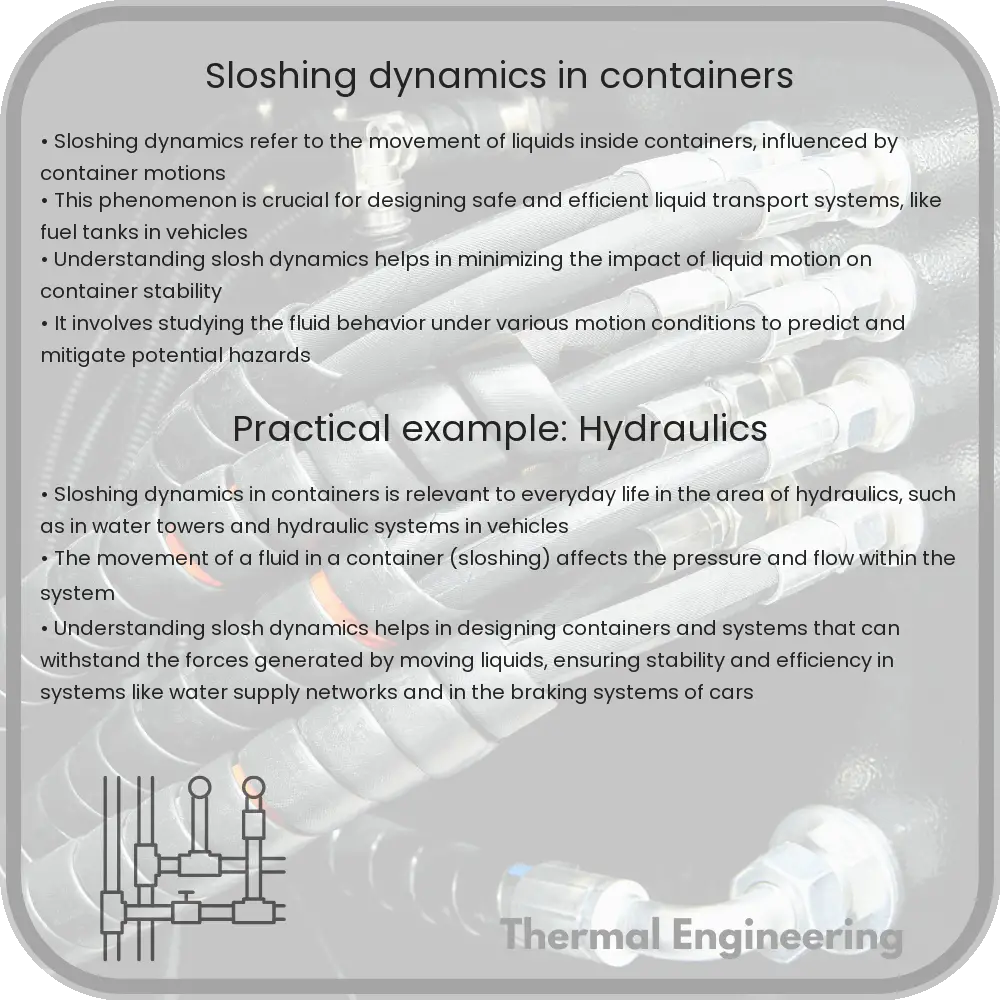
Sloshing refers to the movement of a liquid inside a partially filled container, which can occur during transportation or any motion of the container. Sloshing can affect the stability of the container and the entire structure it supports, such as a cargo ship or a tanker truck. Understanding the dynamics of sloshing is crucial for the design and safety of these transport systems.

Factors Influencing Sloshing

Sloshing dynamics can be influenced by several factors including:

• The fluid properties, such as density and viscosity.
• The fill level of the container.
• The shape and dimensions of the container.
• The amplitude and frequency of the external forcing.

The interaction between these factors can lead to complex fluid motions and forces exerted on the container walls.

Mathematical Modeling of Sloshing

The mathematical description of sloshing typically involves the potential flow theory, where the fluid is considered inviscid (having no viscosity) and incompressible. The Navier-Stokes equations, which describe the motion of viscous fluid substances, can be simplified under these assumptions.

For small amplitude oscillations, the sloshing in containers can be approximately modeled by the linear wave equation:

\[ h(x,t) = \sum A_n \sin(n \pi \frac{x}{L}) \cos(\omega_n t) \]

where:

• \( h(x,t) \) is the height of the liquid surface above the rest position.
• \( A_n \) are the amplitudes of the modes.
• \( n \) is the mode number.
• \( L \) is the length of the tank.
• \( \omega_n \) is the natural frequency of the \( n^{th} \) mode.

The natural frequencies \(\omega_n\) are particularly important and can be calculated as:

\[ \omega_n = \sqrt{\frac{n^2 \pi^2 g}{L}} \]

where \( g \) is the acceleration due to gravity.

Practical Considerations and Safety

Understanding and predicting sloshing is essential for the safe design of liquid-carrying vehicles and tanks. Measures such as baffles or changes in container geometry can be used to mitigate the sloshing effects. For accurate predictions, more sophisticated computational fluid dynamics (CFD) simulations are usually required.

CFD simulations consider complex aspects like the exact fluid properties, detailed geometries, and non-linear interactions which are beyond the scope of simple analytical models.

Application in Real-World Designs

The principles of sloshing dynamics are applied in various engineering fields:

• Automotive engineering, for the design of fuel tanks in vehicles.
• Shipbuilding, where liquid cargo can significantly impact the stability of the ship.
• Civil engineering, for designing water towers and other liquid containers that can be subjected to environmental forces.

By incorporating sloshing dynamics into their designs, engineers can enhance stability, efficiency, and safety of systems that involve liquid storage and transport.

In conclusion, sloshing dynamics is a fascinating area of fluid mechanics with significant applications in engineering. The ability to predict sloshing behavior is key to designing safer and more efficient systems that face the challenges of liquid motion.

Learn about flow-induced vibration in pipes, a critical issue affecting the safety and integrity of piping systems in various industries.

Understanding Flow-Induced Vibration in Pipes

Flow-induced vibration (FIV) in piping systems is a critical phenomenon that occurs when the fluid flow within pipes causes the pipes themselves to vibrate. These vibrations, if not adequately controlled or monitored, can lead to fatigue failures or other significant damage to the piping system and associated machinery. Understanding the basics of FIV is essential for engineers to design more reliable and safer piping systems.

Causes of Flow-Induced Vibration

There are several mechanisms by which flow can induce vibrations in pipes:

• Vortex Shedding: As fluid flows past a blunt body (such as a pipe), vortices are formed alternately on both sides of the body, creating oscillating pressures that can lead to vibration. The frequency of these vibrations is known as the shedding frequency and depends on the flow velocity, the diameter of the pipe, and the fluid’s properties.
• Acoustic Resonance: This occurs when the pressure waves generated by the flow resonate with the natural frequency of the pipe system, leading to potentially high vibration and noise levels.
• Fluidelastic Instability: In systems with arrays of tubes (e.g., heat exchangers), fluid flow can cause an instability where tubes start to vibrate excessively in a fluid flow field. This is often considered the most severe form of FIV in heat exchanger tube arrays.
• Turbulence: High levels of turbulence in the flow can exert random fluctuating forces on the walls of the pipes, leading to vibrations.

Effects of Flow-Induced Vibration

The effects of unmanaged FIV are largely detrimental to the piping infrastructure:

• Pipe Fatigue: Repeated vibration can lead to fatigue in pipes, eventually causing cracks and failures.
• Loosening of Joints: Vibrational forces can loosen the joints and connections in pipe systems, leading to leaks or catastrophic failures.
• Noise: Vibrations can propagate through structures as sound, creating noise that can be hazardously loud in industrial environments.
• Wear and Tear: Continuous vibration increases the wear and tear on supporting structures and dampers.

Controlling Flow-Induced Vibration

It is essential to control FIV to maintain the integrity and longevity of piping systems. Common measures include:

• Proper Support and Damping: Providing adequate supports and using damping mechanisms can reduce the amplitude of vibrations.
• Optimizing Flow Conditions: Adjusting the velocity of the fluid and redesigning the pipe system to avoid resonance conditions can help avoid FIV.
• Vibration Monitoring: Continuous monitoring using vibration sensors can help detect potential problems early before they lead to system failure.

Conclusion

Flow-induced vibration in pipes is a complex issue that encompasses fluid dynamics, materials science, and structural engineering. Effective management of FIV is key to ensuring the safety and efficiency of various industrial operations. As technologies advance, more sophisticated methods for predicting, detecting, and mitigating FIV continue to be developed, offering greater safety and reliability in fluid handling systems.

Learn about wave breaking, a key natural process influencing oceanography, coastal engineering, and weather prediction, through its types, physics, and environmental impact.

Understanding Wave Breaking Phenomena

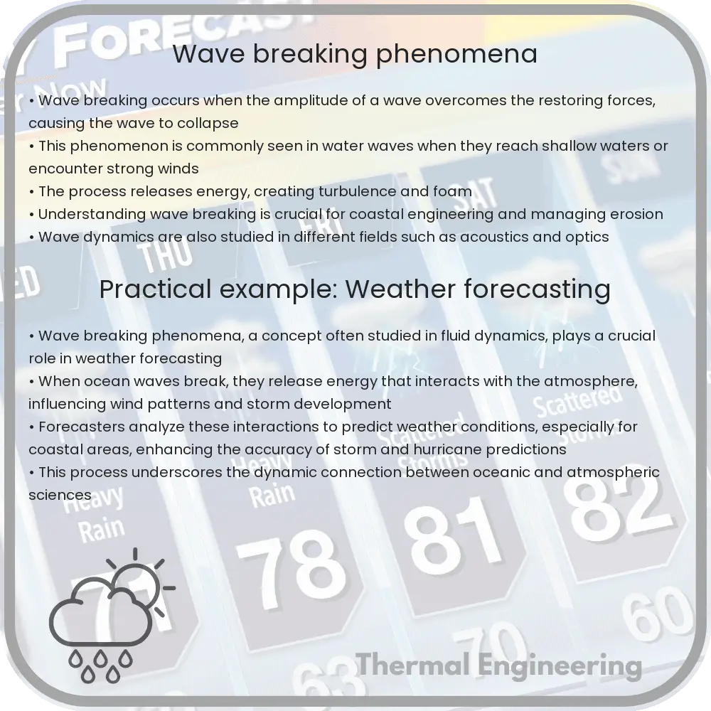
Wave breaking is a fascinating natural phenomenon that occurs when the crest of a water wave topples over onto itself. This process is crucial in various disciplines, including oceanography, coastal engineering, and environmental science. The understanding of wave breaking helps in designing coastal structures, predicting weather patterns, and studying marine ecosystems.

Types of Wave Breaking

Wave breaking can be classified into three main types:

1. Spilling Breakers: These occur when the base of the wave moves faster than the crest, causing the wave to gently spill. They are common on gradually sloping beaches and release energy slowly over a longer distance.
2. Plunging Breakers: Characterized by the dramatic curl of the wave crest, plunging breakers are typical on moderately steep slopes. These waves crash down with considerable energy and are popular with surfers.
3. Surging Breakers: These waves occur on steep shores and do not actually break as they approach the shore. Instead, they surge upward and the wave face maintains its integrity as it runs up the beach.

Physics of Wave Breaking

The simplest theoretical description of wave breaking dynamics involves the balance of gravitational forces against the surface tension of the water. The onset of breaking occurs when the steepness (the ratio of wave height, \(H\), to wavelength, \(L\)) of a wave reaches a critical threshold. The Rayleigh Instability Criterion can predict this, which suggests wave breaking initiates when the wave crest speed exceeds the wave celerity (wave speed).

Mathematically, this is given by:

\[
\frac{H}{L} > \frac{1}{7}
\]

This equation indicates that when the wave height is more than one-seventh of the wave length, breaking is likely to occur.

Impact of Wave Breaking

Wave breaking is not just a visually spectacular phenomenon; it has profound effects on the coastal and marine environment:

• Energy Dissipation: Breaking waves are primary agents in the dissipation of ocean surface wave energy. The energy lost during breaking contributes to coastal erosion and the mixing of upper layers of the ocean, affecting marine life habitats and nutrient distribution.
• Aeration and Gas Exchange: As waves break, they trap air, forming bubble clouds that significantly enhance the oxygenation of the water and promote gas exchanges between the ocean and atmosphere.
• Sound Generation: Breaking waves generate sound waves which can be used in various research fields to study the properties of near-shore environments.

Conclusion

The study of wave breaking phenomena is essential in our understanding of coastal environments and marine dynamics. Engineers and scientists continue to explore these processes, seeking enhanced models that can better predict their behavior under different conditions. As our understanding improves, so too does our ability to protect coastal infrastructures and manage marine resources efficiently.

Whether it’s the gentle roll of a spilling breaker or the dramatic crash of a plunging wave, each breaking wave tells a story of energy, motion, and the delicate balance of forces that govern them.

Explore how air quality modeling assesses and manages urban air pollution, using data and simulations to predict pollutant dispersion.

Understanding Air Quality Modeling in Urban Areas

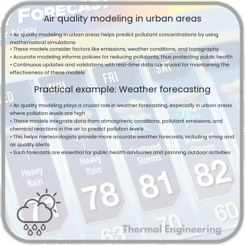
Air quality modeling serves as a crucial tool in assessing the health of the urban environment and managing public health risks related to air pollution. Urban areas, with their high density of vehicles, industrial activities, and energy production, are particularly susceptible to air pollution. Air quality models help predict the dispersion of pollutants and their concentration in the air over time, enabling city planners and public health officials to make informed decisions.

How Air Quality Modeling Works

Air quality modeling involves using mathematical and computational techniques to simulate the physical and chemical processes that pollutants undergo as they diffuse through the atmosphere. These models typically intake data such as emissions from various sources, meteorological conditions, and topography to predict pollutant levels.

Types of Air Quality Models

• Gaussian models: These models are based on the Gaussian plume equation, which assumes that the pollutants disperse in the air in a bell-shaped curve. They are widely used for estimating the dispersion of pollutants from single sources, such as factory chimneys.
• Grid models (Eulerian models): These models divide the air space into a three-dimensional grid and solve the pollutant dispersion equations for each cell. The approach is useful for more complex scenarios involving multiple interacting pollution sources and varying meteorological conditions.
• Lagrangian models: These models track the movement of air parcels as they move through the environment, accounting for changes in pollutant concentrations due to chemical reactions and interactions with the earth’s surface. This type is particularly useful for studying long-range transport of pollutants.

Key Equations in Air Quality Modeling

The general dispersion equation critical to most air quality models can be given by:

∆C / ∆t = -U * (∆C / ∆x) – V * (∆C / ∆y) – W * (∆C / ∆z) + S + E

• ∆C / ∆t is the rate of change of pollutant concentration.
• U, V, W are the wind speeds in the x, y, and z directions, respectively.
• ∆x, ∆y, ∆z represent changes in space along the x, y, and z axes.
• S represents the sources of pollution.
• E represents the environmental loss terms, including deposition and chemical reaction.

The Role of Data in Air Quality Modeling

Accurate data is the backbone of effective air quality modeling. Inputs commonly used include:

1. Emissions data: Information on the types and quantities of pollutants released by various sources.
2. Meteorological data: Details about wind speed and direction, temperature, humidity, and solar radiation, which influence pollutant dispersion and chemical reactions.
3. Topographic data: Landscape features that affect air flow and pollutant distribution, such as hills, buildings, and bodies of water.

Implications and Applications

Air quality models are not just academic tools; they have practical applications in urban planning and public health. They are used to:

• Forecast air pollution levels, helping to alert populations to unhealthy conditions in advance.
• Develop air pollution control strategies, assessing the potential impact of proposed industrial developments or traffic management schemes.
• Identify hotspots of high pollution for targeted action.
• Contribute to environmental impact assessments required for new projects.

Overall, air quality modeling is an indispensable method in the toolkit of modern urban planning and environmental management, helping mitigate one of the most pressing issues faced by cities around the world—air pollution.

Computational Fluid Dynamics (CFD) is used to optimize wind turbine design by simulating air flow around structures, enhancing performance and efficiency.

Understanding CFD in Wind Turbine Design

Computational Fluid Dynamics (CFD) is a crucial tool in the engineering analysis and design of wind turbines. By simulating how the air flows around and through wind turbine structures, CFD helps engineers optimize performance, durability, and efficiency. In this article, we will explore the basics of CFD, its role in wind turbine design, and how it contributes to enhancing the energy production capabilities of wind turbines.

What is Computational Fluid Dynamics (CFD)?

CFD is a branch of fluid mechanics that uses numerical analysis and data structures to solve and analyze problems involving fluid flows. Computers are used to perform the calculations required to simulate the interaction of liquids and gases with surfaces defined by boundary conditions. The impact of CFD in industrial applications is significant, as it allows for the detailed visual analysis of how a fluid flows and how it affects objects in its path.

Key Benefits of CFD in Wind Turbine Design

• Performance Optimization: CFD analysis aids in the study of airflow patterns around the turbine blades, helping to optimize the blade shape and configuration for maximum efficiency.
• Structural Analysis: It helps analyze the strain and stress on the structures of the turbine to predict and prevent possible failure points.
• Acoustic Analysis: Engineers can use CFD to simulate and mitigate the noise production of wind turbines, which is critical for compliance with environmental standards and for installations near residential areas.

CFD Process in Wind Turbine Design

The process of applying CFD in wind turbine design generally involves several steps:

1. Geometry Creation: A 3D model of the wind turbine components (e.g., rotor blade, nacelle) is created.
2. Meshing: The model is divided into smaller, discrete cells in a mesh. The quality of the mesh significantly affects the accuracy and stability of the CFD simulation.
3. Setting Up Boundary Conditions: Boundary conditions are defined, including the speed, temperature, and pressure of the incoming airflow.
4. Simulation: The CFD simulation is run using the defined settings. The software calculates fluid flow around the 3D model and predicts how the turbine will perform in real-world conditions.
5. Analysis: Data from the simulation is analyzed to assess the performance and robustness of the turbine design. Adjustments and optimizations may be suggested based on the findings.

Challenges and Considerations

While CFD provides a powerful tool for the design and improvement of wind turbines, there are challenges and considerations that must be kept in mind:

• Computational Costs: High-fidelity CFD simulations require significant computational resources and time, making them expensive.
• Accuracy: The accuracy of a CFD simulation is highly dependent on the choice of model, mesh quality, and boundary conditions. Appropriate validations against real-world data are crucial.
• Sensitivity: CFD results can be sensitive to changes in input parameters, requiring careful setup and analysis.

Future Directions

Advancements in CFD technology continue to expand its capabilities and reduce costs associated with its use in wind turbine design. Ongoing research focuses on improving the accuracy of CFD simulations and integrating them with other simulation methods to create comprehensive models that can predict overall turbine performance under various conditions.

As CFD tools become more accessible and integrated into engineering workflows, their role in the design and optimization of wind turbines is likely to grow, leading to more efficient, reliable, and cost-effective wind energy solutions.

A detailed exploration of thermal desalination technologies, their principles, types, applications, and future advancements.

Understanding Thermal Desalination Technologies

Desalination refers to the process of removing salts and other minerals from saline water to produce water suitable for human consumption or irrigation. Among the various methods employed for desalination, thermal desalination technologies stand out due to their reliance on heat to separate water from salts. This article explores the principle, types, and applications of thermal desalination technologies.

Principle of Thermal Desalination

The basic principle behind thermal desalination is the use of heat to evaporate water, leaving salts and other impurities behind in the remaining brine. The vapor is then condensed to produce fresh water. This process leverages the different boiling points of water and the dissolved salts, a method known scientifically as phase change.

Types of Thermal Desalination Technologies

• Multi-Stage Flash Distillation (MSF): MSF involves heating saline water and then allowing it to boil in multiple stages or ‘flashes’ under lower and lower pressures. Each subsequent flash operates at a lower pressure which allows boiling at lower temperatures, utilizing the latent heat released from the previous stages to improve efficiency. MSF is widely used, particularly in the Middle East where energy costs are relatively low.
• Multiple Effect Distillation (MED): In MED, saline water is also heated and then passed through multiple effects where it is evaporated and condensed in a series of stages at decreasing pressures and temperatures. Unlike MSF, MED captures and reuses the heat of condensation from each effect to preheat incoming saline water into the next effect, making it slightly more energy-efficient than MSF.
• Vapor Compression (VC): Vapor Compression desalination uses a mechanical compressor or thermal vapor compressor to compress the vapor produced by boiling saline water. The compression increases the vapor temperature, allowing it to be used as an efficient heat source for boiling more water. VC can be either Mechanical Vapor Compression (MVC) or Thermal Vapor Compression (TVC), depending on the compression process.

Applications and Advantages

Thermal desalination technologies are predominantly used in regions where energy resources are abundant and inexpensive since these processes are energy-intensive. The primary application of these technologies is the provision of potable water in arid regions or places where freshwater sources are limited. They are particularly crucial in the Middle East and North Africa (MENA) region.

One of the main advantages of thermal desalination methods is their robustness and reliability, able to handle high saline concentrations and larger capacities, making them suitable for municipal and industrial scales. Furthermore, they feature relatively simpler technology compared to other desalination processes like Reverse Osmosis (RO), making them less prone to fouling and scaling.

Challenges and Future Directions

Despite their advantages, thermal desalination technologies face significant challenges, primarily related to their high energy consumption and environmental impact. The disposal of brine, which is high in salt concentration and often contains other chemicals, poses serious environmental consequences. Moreover, the heavy reliance on fossil fuels raises concerns about carbon emissions and sustainability.

Future advancements in thermal desalination technologies focus on integrating renewable energy sources, like solar or wind power, to decrease dependency on non-renewable resources. Innovative approaches such as using low-grade heat from industrial processes or geothermal sources are also being explored to enhance the energy efficiency of these systems.

While thermal desalination technologies are amongst the oldest and most established methods for producing freshwater, constant innovation is necessary to address their environmental and economic challenges, making desalination a more sustainable solution for water scarcity.

Conclusion

Thermal desalination technologies play a vital role in addressing global water scarcity issues by providing a dependable method for producing potable water from the sea. While they offer several benefits in terms of reliability and capacity, the challenge lies in making these technologies more energy-efficient and environmentally friendly. As research continues and technology advances, thermal desalination is poised to become an even more critical component in the global water supply strategy.

Geophysical fluid dynamics explores natural fluid flows on Earth, aiding in understanding climate patterns and changes.

Understanding Geophysical Fluid Dynamics in Climate Studies

Geophysical fluid dynamics (GFD) is a fundamental branch of fluid mechanics that deals with the natural flows occurring on Earth and other celestial bodies. It encompasses the study of both atmospheric and oceanic motion driven by forces such as gravity, Coriolis effect, and thermal gradients. Importantly, this field plays a vital role in climate studies, offering insights into how these large-scale fluid flows affect weather, climate patterns, and ultimately global climate change.

The Basics of Geophysical Fluid Dynamics

The study of GFD focuses on the complex interactions between fluid flows and the forces acting on them. Some key forces include:

• Gravity: Causes fluids to flow downhill and influences oceanic and atmospheric circulations through density variations.
• Pressure gradients: Drive fluids from high to low pressure areas, crucial in shaping weather patterns and ocean currents.
• Coriolis effect: A result of Earth’s rotation, impacting the direction of fluid flows and leading to phenomena such as trade winds and the Gulf Stream.
• Solar radiation: Affects temperature, driving thermal expansions and contractions in the atmosphere and oceans, thus influencing circulation patterns.

GFD also involves the formulation and solving of the Navier-Stokes equations under the influence of these forces. These equations describe how the velocity field of fluid flows evolves in response to various forces and are expressed as:

i. Continuity equation (mass conservation):

\[\nabla \cdot \vec{v} = 0\]

ii. Momentum equation (force balance):

\[\frac{\partial \vec{v}}{\partial t} + (\vec{v} \cdot \nabla)\vec{v} = -\frac{1}{\rho}\nabla p + \nu \nabla^2 \vec{v} + \vec{f}\]

where \(\vec{v}\) represents the velocity field, \(p\) is pressure, \(\rho\) is density, \(\nu\) is viscosity, and \(\vec{f}\) includes external forces such as gravity and Coriolis force.

Application of GFD in Climate Studies

One critical application of GFD in climate studies is in the development and refinement of climate models. These models are essential for predicting future climate patterns and understanding potential impacts of climate change. GFD helps model how heat and carbon are transported in the atmosphere and oceans, influencing global temperatures and weather extremes.

Moreover, GFD is integral in studying phenomena like El Niño and La Niña, which have profound effects on global weather. The dynamics of these events, involving interactions between ocean and atmosphere, are governed by the principles of GFD.

Through satellite data and supercomputers, researchers can implement GFD to simulate flows on the global scale, improving the accuracy of weather forecasting and climate projections. Advances in computational fluid dynamics (CFD) have also enhanced the resolution and accuracy of these models, enabling more detailed and comprehensive climate analysis.

Challenges and Future Directions

Despite notable advances, there remain challenges in GFD, particularly relating to the scale and complexity of climate systems. Issues such as turbulent flows and chaotic system behavior present difficulties in accurately predicting long-term climate changes. Researchers continue to refine methods to handle these complexities, integrating data from multiple sources and utilizing increasingly powerful computational resources.

The future of GFD in climate studies will likely focus on improving multi-scale models and enhancing our understanding of feedback mechanisms between different components of the Earth system. As we continue to witness the unfolding impacts of climate change, the role of GFD will undoubtedly remain essential in devising strategies to mitigate and adapt to these changes effectively.

The intersection of GFD with advanced technology and interdisciplinary research holds the promise of yielding deeper insights into the complexities of our planet’s climate, contributing significantly to sustaining Earth’s environment for future generations.