Turbulent Flow
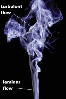
In fluid dynamics, turbulent flow is characterized by the irregular movement of particles (one can say chaotic) of the fluid. In contrast to laminar flow the fluid does not flow in parallel layers, the lateral mixing is very high, and there is a disruption between the layers. Turbulence is also characterized by recirculation, eddies, and apparent randomness. In turbulent flow the speed of the fluid at a point is continuously undergoing changes in both magnitude and direction.
Detailed knowledge of behaviour of turbulent flow regime is of importance in engineering, because most industrial flows, especially those in nuclear engineering are turbulent. Unfortunately, the highly intermittent and irregular character of turbulence complicates all analyses. In fact, turbulence is often said to be the “last unsolved problem in classical mathemetical physics.”
The main tool available for their analysis is CFD analysis. CFD is a branch of fluid mechanics that uses numerical analysis and algorithms to solve and analyze problems that involve turbulent fluid flows. It is widely accepted that the Navier–Stokes equations (or simplified Reynolds-averaged Navier–Stokes equations) are capable of exhibiting turbulent solutions, and these equations are the basis for essentially all CFD codes.
See also: Internal Flow
See also: External Flow
Characteristics of Turbulent Flow
- Turbulent flow tends to occur at higher velocities, low viscosity and at higher characteristic linear dimensions.
- If the Reynolds number is greater than Re > 3500, the flow is turbulent.
- Irregularity: The flow is characterized by the irregular movement of particles of the fluid. The movement of fluid particles is chaotic. For this reason, turbulent flow is normally treated statistically rather than deterministically.
- Diffusivity: In turbulent flow, a fairly flat velocity distribution exists across the section of pipe, with the result that the entire fluid flows at a given single value and drops rapidly extremely close to the walls. The characteristic which is responsible for the enhanced mixing and increased rates of mass, momentum and energy transports in a flow is called “diffusivity”.
- Rotationality: Turbulent flow is characterized by a strong three-dimensional vortex generation mechanism. This mechanism is known as vortex stretching.
- Dissipation: A dissipative process is a process in which the kinetic energy of turbulent flow is transformed into internal energy by viscous shear stress.
Reynolds Number
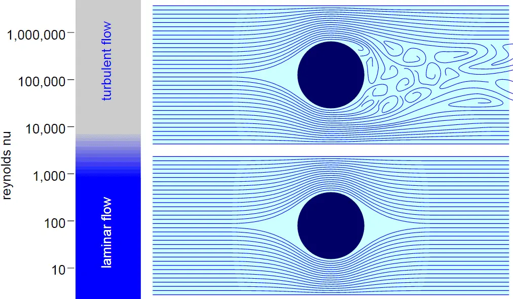
The Reynolds number is the ratio of inertial forces to viscous forces and is a convenient parameter for predicting if a flow condition will be laminar or turbulent. It can be interpreted that when the viscous forces are dominant (slow flow, low Re) they are sufficient enough to keep all the fluid particles in line, then the flow is laminar. Even very low Re indicates viscous creeping motion, where inertia effects are negligible. When the inertial forces dominate over the viscous forces (when the fluid is flowing faster and Re is larger) then the flow is turbulent.
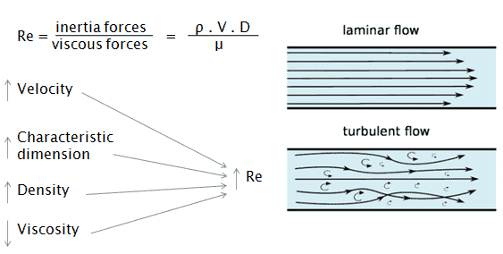
It is a dimensionless number comprised of the physical characteristics of the flow. An increasing Reynolds number indicates an increasing turbulence of flow.
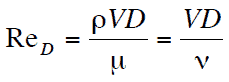
It is defined as:
where:
V is the flow velocity,
D is a characteristic linear dimension, (travelled length of the fluid; hydraulic diameter etc.)
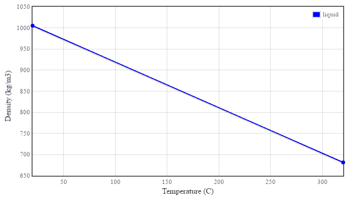
ρ fluid density (kg/m3),
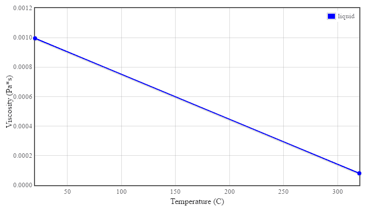
μ dynamic viscosity (Pa.s),
ν kinematic viscosity (m2/s); ν = μ / ρ.
Laminar vs. Turbulent Flow
Laminar flow:
- Re < 2000
- ‘low’ velocity
- Fluid particles move in straight lines
- Layers of water flow over one another at different speeds with virtually no mixing between layers.
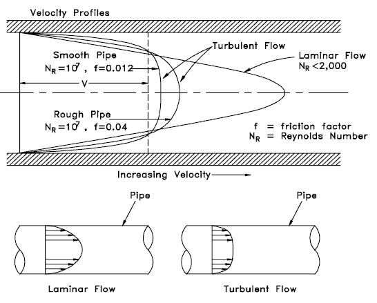
- The flow velocity profile for laminar flow in circular pipes is parabolic in shape, with a maximum flow in the center of the pipe and a minimum flow at the pipe walls.
- The average flow velocity is approximately one half of the maximum velocity.
- Simple mathematical analysis is possible.
- Rare in practice in water systems.
Turbulent Flow:
- Re > 4000
- ‘high’ velocity
- The flow is characterized by the irregular movement of particles of the fluid.
- Average motion is in the direction of the flow
- The flow velocity profile for turbulent flow is fairly flat across the center section of a pipe and drops rapidly extremely close to the walls.
- The average flow velocity is approximately equal to the velocity at the center of the pipe.
- Mathematical analysis is very difficult.
- Most common type of flow.
Source: Blevins, R. D. (1990), Flow Induced Vibration, 2nd Edn., Van Nostrand Reinhold Co.
All fluid flow is classified into one of two broad categories or regimes. These two flow regimes are:
- Single-phase Fluid Flow
- Multi-phase Fluid Flow (or Two-phase Fluid Flow)
This is a basic classification. All of the fluid flow equations (e.g. Bernoulli’s Equation) and relationships that were discussed in this section (Fluid Dynamics) were derived for the flow of a single phase of fluid whether liquid or vapor. Solution of multi-phase fluid flow is very complex and difficult and therefore it is usually in advanced courses of fluid dynamics.
 Another usually more common classification of flow regimes is according to the shape and type of streamlines. All fluid flow is classified into one of two broad categories. The fluid flow can be either laminar or turbulent and therefore these two categories are:
- Laminar Flow
- Turbulent Flow
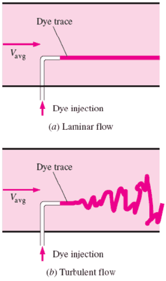
Laminar flow is characterized by smooth or in regular paths of particles of the fluid. Therefore the laminar flow is also referred to as streamline or viscous flow. In contrast to laminar flow, turbulent flow is characterized by the irregular movement of particles of the fluid. The turbulent fluid does not flow in parallel layers, the lateral mixing is very high, and there is a disruption between the layers. Most industrial flows, especially those in nuclear engineering are turbulent.
The flow regime can be also classified according to the geometry of a conduit or flow area. From this point of view, we distinguish:
- Internal Flow
- External Flow
Internal flow is a flow for which the fluid is confined by a surface. Detailed knowledge of behaviour of internal flow regimes is of importance in engineering, because circular pipes can withstand high pressures and hence are used to convey liquids. On the other hand, external flow is such a flow in which boundary layers develop freely, without constraints imposed by adjacent surfaces. Detailed knowledge of behaviour of external flow regimes is of importance especially in aeronautics and aerodynamics.
 Laminar flow. For practical purposes, if the Reynolds number is less than 2000, the flow is laminar. The accepted transition Reynolds number for flow in a circular pipe is Red,crit = 2300.
Transitional flow. At Reynolds numbers between about 2000 and 4000 the flow is unstable as a result of the onset of turbulence. These flows are sometimes referred to as transitional flows.
Turbulent flow. If the Reynolds number is greater than 3500, the flow is turbulent. Most fluid systems in nuclear facilities operate with turbulent flow.
Turbulent Velocity Profile
Power-law velocity profile – Turbulent velocity profile
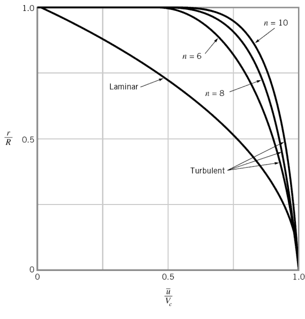
 The velocity profile in turbulent flow is flatter in the central part of the pipe (i.e. in the turbulent core) than in laminar flow. The flow velocity drops rapidly extremely close to the walls. This is due to the diffusivity of the turbulent flow.
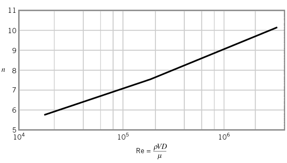
In case of turbulent pipe flow, there are many empirical velocity profiles. The simplest and the best known is the power-law velocity profile:
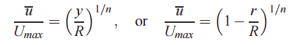
where the exponent n is a constant whose value depends on the Reynolds number. This dependency is empirical and it is shown at the picture. In short, the value n increases with increasing Reynolds number. The one-seventh power-law velocity profile approximates many industrial flows.
Examples of Turbulent Flow
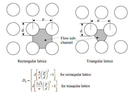
Inside the reactor pressure vessel of PWR, the coolant first flows down outside the reactor core (through the downcomer). From the bottom of the pressure vessel, the flow is reversed up through the core, where the coolant temperature increases as it passes through the fuel rods and the assemblies formed by them. The Reynolds number inside the fuel channel is equal to:
ReDH = 5 [m/s] x 0.01 [m] / 0.12×10⁻⁶ [m2/s] = 416 600.
This also fully satisfies the turbulent conditions.
See also: Hydraulic Diameter
 For the first few centimeters, the flow is certainly laminar. However, at some point from the leading edge the flow will naturally transition to turbulent flow as its Reynolds number increases. The Reynolds number increases as its flow velocity and characteristic length are both increasing.
Turbulent Boundary Layer
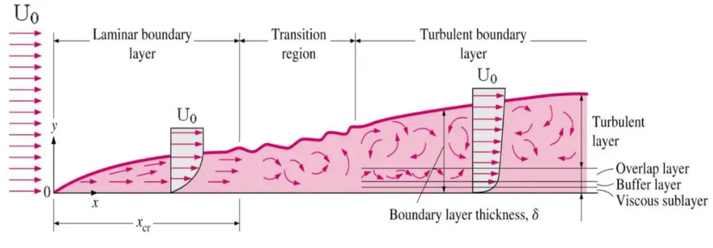
The concept of boundary layers is of importance in all of viscous fluid dynamics, aerodynamics, and also in the theory of heat transfer. Basic characteristics of all laminar and turbulent boundary layers are shown in the developing flow over a flat plate. The stages of the formation of the boundary layer are shown in the figure below:
Boundary layers may be either laminar, or turbulent depending on the value of the Reynolds number. Also here the Reynolds number represents the ratio of inertia forces to viscous forces and is a convenient parameter for predicting if a flow condition will be laminar or turbulent. It is defined as:
in which V is the mean flow velocity, D a characteristic linear dimension, ρ fluid density, μ dynamic viscosity, and ν kinematic viscosity.
For lower Reynolds numbers, the boundary layer is laminar and the streamwise velocity changes uniformly as one moves away from the wall, as shown on the left side of the figure. As the Reynolds number increases (with x) the flow becomes unstable and finally for higher Reynolds numbers, the boundary layer is turbulent and the streamwise velocity is characterized by unsteady (changing with time) swirling flows inside the boundary layer.
Transition from laminar to turbulent boundary layer occurs when Reynolds number at x exceeds Rex ~ 500,000. Transition may occur earlier, but it is dependent especially on the surface roughness. The turbulent boundary layer thickens more rapidly than the laminar boundary layer as a result of increased shear stress at the body surface.
See also: Boundary layer thickness
See also: Tube in crossflow – external flow
Special reference: Schlichting Herrmann, Gersten Klaus. Boundary-Layer Theory, Springer-Verlag Berlin Heidelberg, 2000, ISBN: 978-3-540-66270-9
Turbulent Flow – Heat Transfer Coefficient
External Turbulent Flow
The average Nusselt number over the entire plate is determined by:
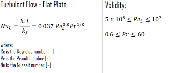
This relation gives the average heat transfer coefficient for the entire plate only when the flow is turbulent over the entire plate, or when the laminar flow region of the plate is too small relative to the turbulent flow region.
Internal Turbulent Flow – Dittus-Boelter
See also: Dittus-Boelter Equation
For fully developed (hydrodynamically and thermally) turbulent flow in a smooth circular tube, the local Nusselt number may be obtained from the well-known Dittus-Boelter equation. The Dittus–Boelter equation is easy to solve but is less accurate when there is a large temperature difference across the fluid and is less accurate for rough tubes (many commercial applications), since it is tailored to smooth tubes.
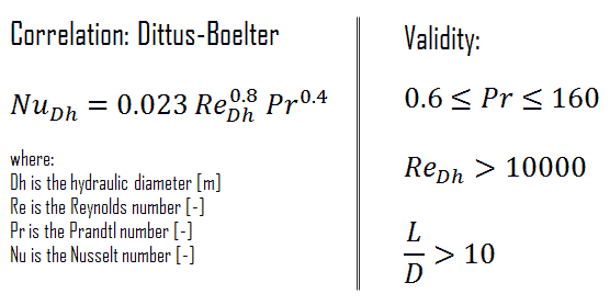
The Dittus-Boelter correlation may be used for small to moderate temperature differences, Twall – Tavg, with all properties evaluated at an averaged temperature Tavg.
For flows characterized by large property variations, the corrections (e.g. a viscosity correction factor μ/μwall) must be taken into account, for example, as Sieder and Tate recommend.
Kolmogorov Microscales
In the view of Kolmogorov (Andrey Nikolaevich Kolmogorov was a Russian mathematician who made significant contributions to the mathematics of probability theory and turbulence), turbulent motions involve a wide range of scales. From a macroscale at which the energy is supplied, to a microscale at which energy is dissipated by viscosity.
For example, consider a cumulus cloud. The macroscale of the cloud can be of the order of kilometers and may grow or persist over long periods of time. Within the cloud, eddies may occur over scales of the order of millimeters. For smaller flows such as in pipes, the microscales may be much smaller. Most of the kinetic energy of the turbulent flow is contained in the macroscale structures. The energy “cascades” from these macroscale structures to microscale structures by an inertial mechanism. This process is known as the turbulent energy cascade.
The smallest scales in turbulent flow are known as the Kolmogorov microscales. These are small enough that molecular diffusion becomes important and viscous dissipation of energy takes place and the turbulent kinetic energy is dissipated into heat.
The smallest scales in turbulent flow, i.e. the Kolmogorov microscales are:
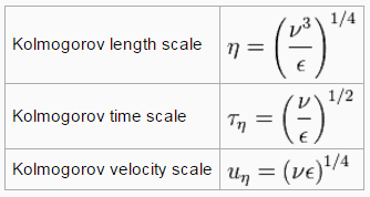
where ε is the average rate of dissipation rate of turbulence kinetic energy per unit mass and has dimensions (m2/s3). ν is the kinematic viscosity of the fluid and has dimensions (m2/s).
The size of the smallest eddy in the flow is determined by viscosity. The Kolmogorov length scale decreases as viscosity decreases. For very high Reynolds number flows, the viscous forces are smaller with respect to inertial forces. Smaller scale motions are then necessarily generated until the effects of viscosity become important and energy is dissipated. The ratio of largest to smallest length scales in the turbulent flow are proportional to the Reynolds number (raises with the three-quarters power).
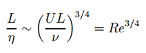
This causes direct numerical simulations of turbulent flow to be practically impossible. For example, consider a flow with a Reynolds number of 106. In this case the ratio L/l is proportional to 1018/4. Since we have to analyze three-dimensional problem, we need to compute a grid that consisted of at least 1014 grid points. This far exceeds the capacity and possibilities of existing computers.
We hope, this article, Turbulent Flow, helps you. If so, give us a like in the sidebar. Main purpose of this website is to help the public to learn some interesting and important information about thermal engineering.