Navier-Stokes Equations
In fluid dynamics, the Navier-Stokes equations are equations, that describe the three-dimensional motion of viscous fluid substances. These equations are named after Claude-Louis Navier (1785-1836) and George Gabriel Stokes (1819-1903). In situations in which there are no strong temperature gradients in the fluid, these equations provide a very good approximation of reality.
The Navier-Stokes equations consists of a time-dependent continuity equation for conservation of mass, three time-dependent conservation of momentum equations and a time-dependent conservation of energy equation. There are four independent variables in the problem, the x, y, and z spatial coordinates of some domain, and the time t.
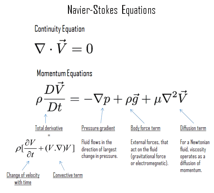
As can be seen, the Navier-Stokes equations are second-order nonlinear partial differential equations, their solutions have been found to a variety of interesting viscous flow problems. They may be used to model the weather, ocean currents, air flow around an airfoil and water flow in a pipe or in a reactor. The Navier–Stokes equations in their full and simplified forms help with the design of aircraft and cars, the study of blood flow, the design of nuclear reactors and many other things.
Solution of Navier-Stokes Equations
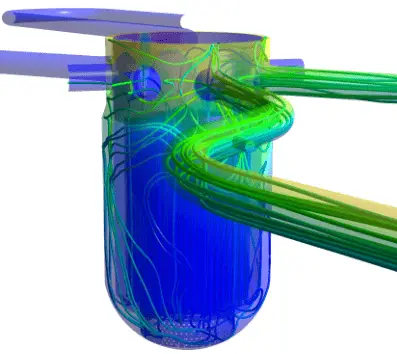
Source: CFD development group – hzdr.de
Even though the Navier-Stokes equations have only a limited number of known analytical solutions, they are amenable to fine-gridded computer modeling. The main tool available for their analysis is CFD analysis. CFD is a branch of fluid mechanics that uses numerical analysis and algorithms to solve and analyze problems that involve turbulent fluid flows. It is widely accepted that the Navier–Stokes equations (or simplified Reynolds-averaged Navier–Stokes equations) are capable of exhibiting turbulent solutions, and these equations are the basis for essentially all CFD codes. It is possible now to achieve approximate, but realistic, CFD results for a wide variety of complex two- and three-dimensional viscous flows.
The Navier–Stokes equations are also of great interest in a purely mathematical sense. Unfortunately, the highly intermittent and irregular character of turbulent flow complicates all analyses. It has not yet been proven that in three dimensions solutions always exist, or that if they do exist, then they are smooth. In fact, general solution of the Navier-Stokes equations with turbulences is often said to be the “last unsolved problem in classical mathemetical physics.”
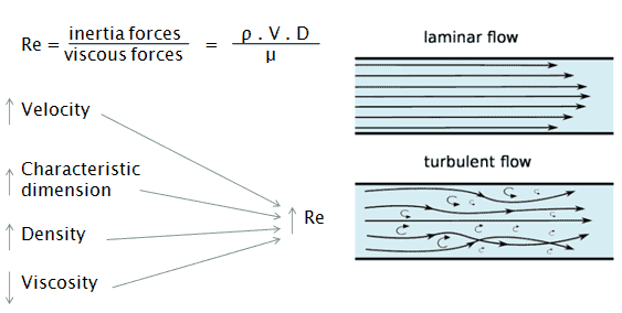
Characteristics of Turbulent Flow
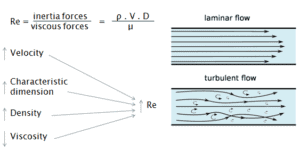 Turbulent flow tends to occur at higher velocities, low viscosity and at higher characteristic linear dimensions.
- If the Reynolds number is greater than Re > 3500, the flow is turbulent.
- Irregularity: The flow is characterized by the irregular movement of particles of the fluid. The movement of fluid particles is chaotic. For this reason, turbulent flow is normally treated statistically rather than deterministically.
- Diffusivity: In turbulent flow, a fairly flat velocity distribution exists across the section of pipe, with the result that the entire fluid flows at a given single value and drops rapidly extremely close to the walls. The characteristic which is responsible for the enhanced mixing and increased rates of mass, momentum and energy transports in a flow is called “diffusivity”.
- Rotationality: Turbulent flow is characterized by a strong three-dimensional vortex generation mechanism. This mechanism is known as vortex stretching.
- Dissipation: A dissipative process is a process in which the kinetic energy of turbulent flow is transformed into internal energy by viscous shear stress.
Kolmogorov Microscales
In the view of Kolmogorov (Andrey Nikolaevich Kolmogorov was a Russian mathematician who made significant contributions to the mathematics of probability theory and turbulence), turbulent motions involve a wide range of scales. From a macroscale at which the energy is supplied, to a microscale at which energy is dissipated by viscosity.
For example, consider a cumulus cloud. The macroscale of the cloud can be of the order of kilometers and may grow or persist over long periods of time. Within the cloud, eddies may occur over scales of the order of millimeters. For smaller flows such as in pipes, the microscales may be much smaller. Most of the kinetic energy of the turbulent flow is contained in the macroscale structures. The energy “cascades” from these macroscale structures to microscale structures by an inertial mechanism. This process is known as the turbulent energy cascade.
The smallest scales in turbulent flow are known as the Kolmogorov microscales. These are small enough that molecular diffusion becomes important and viscous dissipation of energy takes place and the turbulent kinetic energy is dissipated into heat.
The smallest scales in turbulent flow, i.e. the Kolmogorov microscales are:
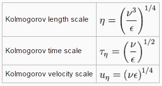
where ε is the average rate of dissipation rate of turbulence kinetic energy per unit mass and has dimensions (m2/s3). ν is the kinematic viscosity of the fluid and has dimensions (m2/s).
The size of the smallest eddy in the flow is determined by viscosity. The Kolmogorov length scale decreases as viscosity decreases. For very high Reynolds number flows, the viscous forces are smaller with respect to inertial forces. Smaller scale motions are then necessarily generated until the effects of viscosity become important and energy is dissipated. The ratio of largest to smallest length scales in the turbulent flow are proportional to the Reynolds number (raises with the three-quarters power).
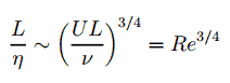
This causes direct numerical simulations of turbulent flow to be practically impossible. For example, consider a flow with a Reynolds number of 106. In this case the ratio L/l is proportional to 1018/4. Since we have to analyze three-dimensional problem, we need to compute a grid that consisted of at least 1014 grid points. This far exceeds the capacity and possibilities of existing computers.
We hope, this article, Navier-Stokes Equation, helps you. If so, give us a like in the sidebar. Main purpose of this website is to help the public to learn some interesting and important information about thermal engineering.