Reynolds Number
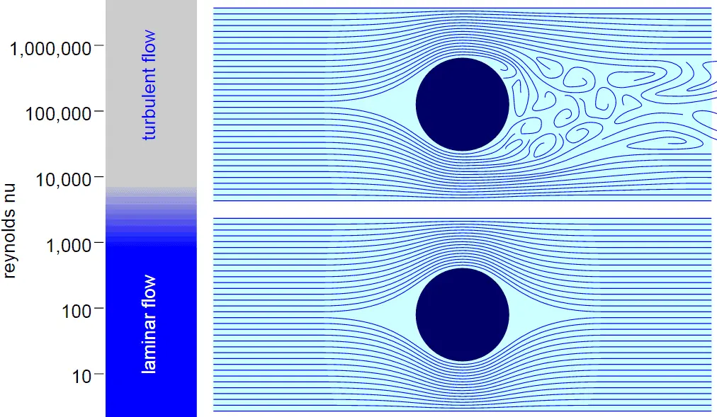
The Reynolds number is the ratio of inertial forces to viscous forces and is a convenient parameter for predicting if a flow condition will be laminar or turbulent. It can be interpreted that when the viscous forces are dominant (slow flow, low Re) they are sufficient enough to keep all the fluid particles in line, then the flow is laminar. Even very low Re indicates viscous creeping motion, where inertia effects are negligible. When the inertial forces dominate over the viscous forces (when the fluid is flowing faster and Re is larger) then the flow is turbulent.
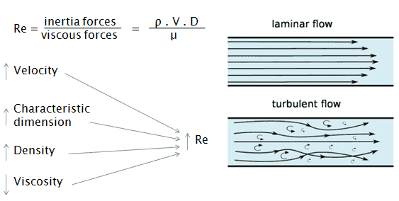
It is a dimensionless number comprised of the physical characteristics of the flow. An increasing Reynolds number indicates an increasing turbulence of flow.
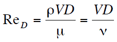
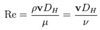
It is defined as:
where:
V is the flow velocity,
D is a characteristic linear dimension, (travelled length of the fluid; hydraulic diameter etc.)
ρ fluid density (kg/m3),
μ dynamic viscosity (Pa.s),
ν kinematic viscosity (m2/s); ν = μ / ρ.
Laminar vs. Turbulent Flow
Laminar flow:
- Re < 2000
- ‘low’ velocity
- Fluid particles move in straight lines
- Layers of water flow over one another at different speeds with virtually no mixing between layers.
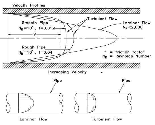
- The flow velocity profile for laminar flow in circular pipes is parabolic in shape, with a maximum flow in the center of the pipe and a minimum flow at the pipe walls.
- The average flow velocity is approximately one half of the maximum velocity.
- Simple mathematical analysis is possible.
- Rare in practice in water systems.
Turbulent Flow:
- Re > 4000
- ‘high’ velocity
- The flow is characterized by the irregular movement of particles of the fluid.
- Average motion is in the direction of the flow
- The flow velocity profile for turbulent flow is fairly flat across the center section of a pipe and drops rapidly extremely close to the walls.
- The average flow velocity is approximately equal to the velocity at the center of the pipe.
- Mathematical analysis is very difficult.
- Most common type of flow.
All fluid flow is classified into one of two broad categories or regimes. These two flow regimes are:
- Single-phase Fluid Flow
- Multi-phase Fluid Flow (or Two-phase Fluid Flow)
This is a basic classification. All of the fluid flow equations (e.g. Bernoulli’s Equation) and relationships that were discussed in this section (Fluid Dynamics) were derived for the flow of a single phase of fluid whether liquid or vapor. Solution of multi-phase fluid flow is very complex and difficult and therefore it is usually in advanced courses of fluid dynamics.
 Another usually more common classification of flow regimes is according to the shape and type of streamlines. All fluid flow is classified into one of two broad categories. The fluid flow can be either laminar or turbulent and therefore these two categories are:
- Laminar Flow
- Turbulent Flow
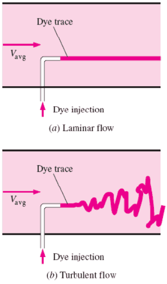
Laminar flow is characterized by smooth or in regular paths of particles of the fluid. Therefore the laminar flow is also referred to as streamline or viscous flow. In contrast to laminar flow, turbulent flow is characterized by the irregular movement of particles of the fluid. The turbulent fluid does not flow in parallel layers, the lateral mixing is very high, and there is a disruption between the layers. Most industrial flows, especially those in nuclear engineering are turbulent.
The flow regime can be also classified according to the geometry of a conduit or flow area. From this point of view, we distinguish:
- Internal Flow
- External Flow
Internal flow is a flow for which the fluid is confined by a surface. Detailed knowledge of behaviour of internal flow regimes is of importance in engineering, because circular pipes can withstand high pressures and hence are used to convey liquids. On the other hand, external flow is such a flow in which boundary layers develop freely, without constraints imposed by adjacent surfaces. Detailed knowledge of behaviour of external flow regimes is of importance especially in aeronautics and aerodynamics.
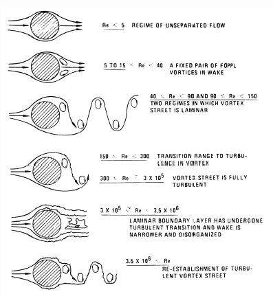
Reynolds Number Regimes
Laminar flow. For practical purposes, if the Reynolds number is less than 2000, the flow is laminar. The accepted transition Reynolds number for flow in a circular pipe is Red,crit = 2300.
Transitional flow. At Reynolds numbers between about 2000 and 4000 the flow is unstable as a result of the onset of turbulence. These flows are sometimes referred to as transitional flows.
Turbulent flow. If the Reynolds number is greater than 3500, the flow is turbulent. Most fluid systems in nuclear facilities operate with turbulent flow.
Reynolds Number and Internal Flow
The internal flow (e.g. flow in a pipe) configuration is a convenient geometry for heating and cooling fluids used in energy conversion technologies such as nuclear power plants.
In general, this flow regime is of importance in engineering, because circular pipes can withstand high pressures and hence are used to convey liquids. Non-circular ducts are used to transport low-pressure gases, such as air in cooling and heating systems.
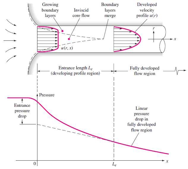
For internal flow regime an entrance region is typical. In this region a nearly inviscid upstream flow converges and enters the tube. To characterize this region the hydrodynamic entrance length is introduced and is approximately equal to:
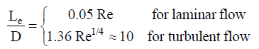
The maximum hydrodynamic entrance length, at ReD,crit = 2300 (laminar flow), is Le = 138d, where D is the diameter of the pipe. This is the longest development length possible. In turbulent flow, the boundary layers grow faster, and Le is relatively shorter. For any given problem, Le / D has to be checked to see if Le is negligible when compared to the pipe length. At a finite distance from the entrance, the entrance effects may be neglected, because the boundary layers merge and the inviscid core disappears. The tube flow is then fully developed.
Power-law velocity profile – Turbulent velocity profile
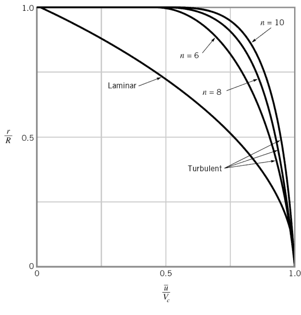
 The velocity profile in turbulent flow is flatter in the central part of the pipe (i.e. in the turbulent core) than in laminar flow. The flow velocity drops rapidly extremely close to the walls. This is due to the diffusivity of the turbulent flow.
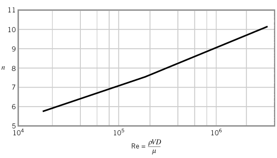
In case of turbulent pipe flow, there are many empirical velocity profiles. The simplest and the best known is the power-law velocity profile:
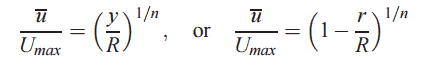
where the exponent n is a constant whose value depends on the Reynolds number. This dependency is empirical and it is shown at the picture. In short, the value n increases with increasing Reynolds number. The one-seventh power-law velocity profile approximates many industrial flows.
Hydraulic Diameter
Since the characteristic dimension of a circular pipe is an ordinary diameter D and especially reactors contains non-circular channels, the characteristic dimension must be generalized.
For these purposes the Reynolds number is defined as:
where Dh is the hydraulic diameter:

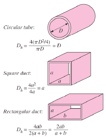 The hydraulic diameter, Dh, is a commonly used term when handling flow in non-circular tubes and channels. The hydraulic diameter transforms non-circular ducts into pipes of equivalent diameter. Using this term, one can calculate many things in the same way as for a round tube. In this equation A is the cross-sectional area, and P is the wetted perimeter of the cross-section. The wetted perimeter for a channel is the total perimeter of all channel walls that are in contact with the flow.
It is an illustrative example, following data do not correspond to any reactor design.
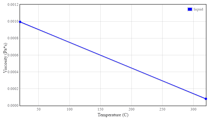
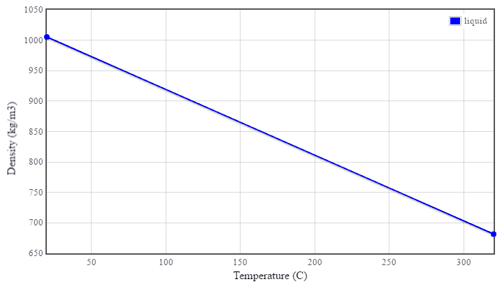
Pressurized water reactors are cooled and moderated by high-pressure liquid water (e.g. 16MPa). At this pressure water boils at approximately 350°C (662°F). Inlet temperature of the water is about 290°C (⍴ ~ 720 kg/m3). The water (coolant) is heated in the reactor core to approximately 325°C (⍴ ~ 654 kg/m3) as the water flows through the core.
The primary circuit of typical PWRs is divided into 4 independent loops (piping diameter ~ 700mm), each loop comprises a steam generator and one main coolant pump. Inside the reactor pressure vessel (RPV), the coolant first flows down outside the reactor core (through the downcomer). From the bottom of the pressure vessel, the flow is reversed up through the core, where the coolant temperature increases as it passes through the fuel rods and the assemblies formed by them.
Assume:
- the primary piping flow velocity is constant and equal to 17 m/s,
- the core flow velocity is constant and equal to 5 m/s,
- the hydraulic diameter of the fuel channel, Dh, is equal to 1 cm
- the kinematic viscosity of the water at 290°C is equal to 0.12 x 10⁻⁶ m2/s
See also: Example: Flow rate through a reactor core
Determine
- the flow regime and the Reynolds number inside the fuel channel
- the flow regime and the Reynolds number inside the primary piping
The Reynolds number inside the primary piping is equal to:
ReD = 17 [m/s] x 0.7 [m] / 0.12×10⁻⁶ [m2/s] = 99 000 000
This fully satisfies the turbulent conditions.
The Reynolds number inside the fuel channel is equal to:
ReDH = 5 [m/s] x 0.01 [m] / 0.12×10⁻⁶ [m2/s] = 416 600
This also fully satisfies the turbulent conditions.
Reynolds Number and External Flow
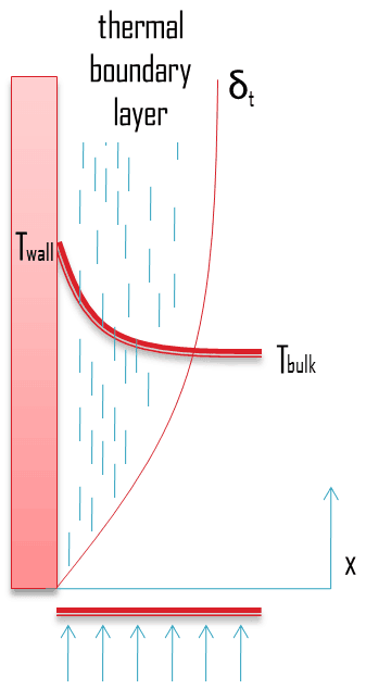
The Reynolds number describes naturally the external flow as well. In general, when a fluid flows over a stationary surface, e.g. the flat plate, the bed of a river, or the wall of a pipe, the fluid touching the surface is brought to rest by the shear stress to at the wall. The region in which flow adjusts from zero velocity at the wall to a maximum in the main stream of the flow is termed the boundary layer.
Basic characteristics of all laminar and turbulent boundary layers are shown in the developing flow over a flat plate. The stages of the formation of the boundary layer are shown in the figure below:
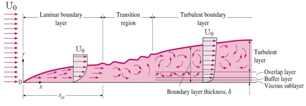
Boundary layers may be either laminar, or turbulent depending on the value of the Reynolds number.
Also here the Reynolds number represents the ratio of inertia forces to viscous forces and is a convenient parameter for predicting if a flow condition will be laminar or turbulent. It is defined as:
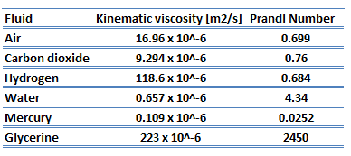
in which V is the mean flow velocity, D a characteristic linear dimension, ρ fluid density, μ dynamic viscosity, and ν kinematic viscosity.
For lower Reynolds numbers, the boundary layer is laminar and the streamwise velocity changes uniformly as one moves away from the wall, as shown on the left side of the figure. As the Reynolds number increases (with x) the flow becomes unstable and finally for higher Reynolds numbers, the boundary layer is turbulent and the streamwise velocity is characterized by unsteady (changing with time) swirling flows inside the boundary layer.
Transition from laminar to turbulent boundary layer occurs when Reynolds number at x exceeds Rex ~ 500,000. Transition may occur earlier, but it is dependent especially on the surface roughness. The turbulent boundary layer thickens more rapidly than the laminar boundary layer as a result of increased shear stress at the body surface.
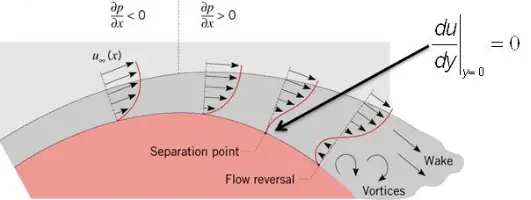
The external flow reacts to the edge of the boundary layer just as it would to the physical surface of an object. So the boundary layer gives any object an “effective” shape which is usually slightly different from the physical shape. We define the thickness of the boundary layer as the distance from the wall to the point where the velocity is 99% of the “free stream” velocity.
To make things more confusing, the boundary layer may lift off or “separate” from the body and create an effective shape much different from the physical shape. This happens because the flow in the boundary has very low energy (relative to the free stream) and is more easily driven by changes in pressure.
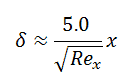
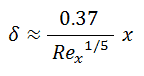
See also: Boundary layer thickness
See also: Tube in crossflow – external flow
Special reference: Schlichting Herrmann, Gersten Klaus. Boundary-Layer Theory, Springer-Verlag Berlin Heidelberg, 2000, ISBN: 978-3-540-66270-9
We hope, this article, Reynolds Number, helps you. If so, give us a like in the sidebar. Main purpose of this website is to help the public to learn some interesting and important information about thermal engineering.