What is Example of Rankine Cycle – Problem with Solution – Definition

Example of Rankine Cycle – Problem with Solution

Let assume the Rankine cycle, which is the one of most common thermodynamic cycles in thermal power plants. In this case assume a simple cycle without reheat  and without with condensing steam turbine running on saturated steam (dry steam). In this case the turbine operates at steady state with inlet conditions of  6 MPa, t = 275.6°C, x = 1 (point 3). Steam leaves this stage of turbine at a pressure of 0.008 MPa, 41.5°C and x = ??? (point 4).

Calculate:

1. the vapor quality of the outlet steam
2. the enthalpy difference between these two states (3 → 4), which corresponds to the work done by the steam, W_T.
3. the enthalpy difference between these two states (1 → 2), which corresponds to the work done by pumps, W_P.
4. the enthalpy difference between these two states (2 → 3), which corresponds to the net heat added in the steam generator
5. the thermodynamic efficiency of this cycle and compare this value with the Carnot’s efficiency

1)

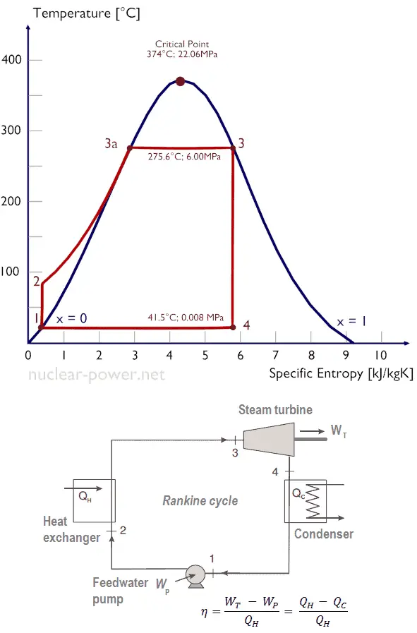
Since we do not know the exact vapor quality of the outlet steam, we have to determine this parameter. State 4 is fixed by the pressure p₄ =  0.008 MPa and the fact that the specific entropy is constant for the isentropic expansion (s₃ = s₄ = 5.89 kJ/kgK for 6 MPa). The specific entropy of saturated liquid water (x=0) and dry steam (x=1) can be picked from steam tables. In case of wet steam, the actual entropy can be calculated with the vapor quality, x, and the specific entropies of saturated liquid water and dry steam:

s₄ = s_v x + (1 – x ) s_l              

where

s₄ = entropy of wet steam (J/kg K) = 5.89 kJ/kgK

s_v = entropy of “dry” steam (J/kg K) = 8.227 kJ/kgK (for 0.008 MPa)

s_l = entropy of saturated liquid water (J/kg K) = 0.592 kJ/kgK (for 0.008 MPa)

From this equation the vapor quality is:

x₄ =  (s₄ – s_l) / (s_v – s_l) = (5.89 – 0.592) / (8.227 – 0.592) = 0.694 = 69.4%

2)

The enthalpy for the state 3 can be picked directly from steam tables, whereas the enthalpy for the state 4 must be calculated using vapor quality:

h_{3, v} = 2785 kJ/kg

h_{4, wet} = h_4,v x + (1 – x ) h_4,l  = 2576 . 0.694 + (1 – 0.694) . 174 = 1787 + 53.2 = 1840 kJ/kg

Then the work done by the steam, W_T, is

W_T = Δh = 945 kJ/kg

3)

Enthalpy for state 1 can be picked directly from steam tables:

h_{1, l} = 174 kJ/kg

State 2 is fixed by the pressure p₂ =  6.0 MPa and the fact that the specific entropy is constant for the isentropic compression (s₁ = s₂ = 0.592 kJ/kgK for 0.008 MPa). For this entropy s₂ = 0.592 kJ/kgK and p₂ =  6.0 MPa we find h_{2, subcooled} in steam tables for compressed water (using interpolation between two states).

h_{2, subcooled} = 179.7 kJ/kg

Then the work done by the pumps, W_P, is

W_P = Δh = 5.7 kJ/kg

4)

The enthalpy difference between (2 → 3), which corresponds to the net heat added in the steam generator, is simply:

Q_add = h_{3, v}  – h_{2, subcooled} = 2785 – 179.7 =  2605.3 kJ/kg

Note that, there is no heat regeneration in this cycle. On the other hand most of the heat added is for the enthalpy of vaporization (i.e. for the phase change).

5)

In this case, steam generators, steam turbine, condensers and feedwater pumps constitute a heat engine, that is subject to the efficiency limitations imposed by the second law of thermodynamics. In the ideal case (no friction, reversible processes, perfect design), this heat engine would have a Carnot efficiency of

η_Carnot = 1 – T_cold/T_hot = 1 – 315/549 = 42.6%

where the temperature of the hot reservoir is 275.6°C (548.7 K), the temperature of the cold reservoir is 41.5°C (314.7K).

The thermodynamic efficiency of this cycle can be calculated by the following formula:

thus
η_th = (945 – 5.7) / 2605.3 = 0.361 = 36.1%

See also:

Rankine Cycle