What is Otto Cycle – pV, Ts Diagram – Definition

Carnot Cycle – pV, Ts diagram

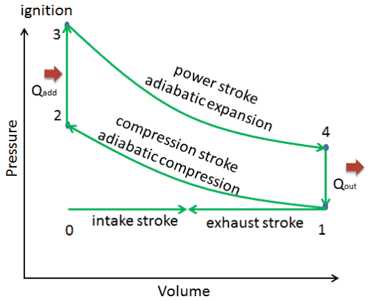
The Otto cycle is often plotted on a pressure- volume diagram (pV diagram) and on a temperature-entropy diagram (Ts diagram). When plotted on a pressure volume diagram, the isochoric processes follow the isochoric lines for the gas (the vertical lines), adiabatic processes move between these vertical lines and the area bounded by the complete cycle path represents the total work that can be done during one cycle.

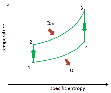
The temperature-entropy diagram (Ts diagram) in which the thermodynamic state is specified by a point on a graph with specific entropy (s) as the horizontal axis and absolute temperature (T) as the vertical axis. Ts diagrams are a useful and common tool, particularly because it helps to visualize the heat transfer during a process. For reversible (ideal) processes, the area under the T-s curve of a process is the heat transferred to the system during that process.

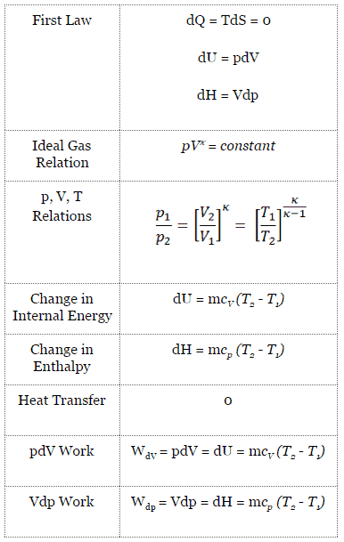
Isentropic Process

An isentropic process is a thermodynamic process, in which the entropy of the fluid or gas remains constant. It means the isentropic process is a special case of an adiabatic process in which there is no transfer of heat or matter. It is a reversible adiabatic process. The assumption of no heat transfer is very important, since we can use the adiabatic approximation only in very rapid processes.

Isentropic Process and the First Law

For a closed system, we can write the first law of thermodynamics in terms of enthalpy:

dH = dQ + Vdp

or

dH = TdS + Vdp

Isentropic process (dQ = 0):

dH = Vdp     →     W = H₂ – H₁     →     H₂ – H₁ = C_p (T₂ – T₁)    (for ideal gas)

Isentropic Process of the Ideal Gas

The isentropic process (a special case of adiabatic process) can be expressed with the ideal gas law as:

pV^κ = constant

or

p₁V₁^κ = p₂V₂^κ

in which κ = c_p/c_v is the ratio of the specific heats (or heat capacities) for the gas. One for constant pressure (c_p) and one for constant volume (c_v). Note that, this ratio κ  = c_p/c_v is a factor in determining the speed of sound in a gas and other adiabatic processes.

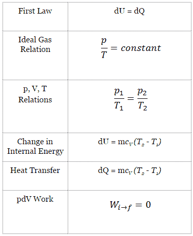
Isothermal Process

An isochoric process is a thermodynamic process, in which the volume of the closed system remains constant (V = const). It describes the behavior of gas inside the container, that cannot be deformed. Since the volume remains constant, the heat transfer into or out of the system does not the p∆V work, but only changes the internal energy (the temperature) of the system.

Isochoric Process and the First Law

The classical form of the first law of thermodynamics is the following equation:

dU = dQ – dW

In this equation dW is equal to dW = pdV and is known as the boundary work. Then:

dU = dQ  – pdV

In isochoric process and the ideal gas, all of heat added to the system will be used to increase the internal energy.

Isochoric process (pdV = 0):

dU = dQ    (for ideal gas)

dU = 0 = Q – W    →     W = Q      (for ideal gas)

Isochoric Process of the Ideal Gas

The isochoric process can be expressed with the ideal gas law as:

or

On a p-V diagram, the process occurs along a horizontal line that has the equation V = constant.

See also: Guy-Lussac’s Law

Comparison of Actual and Ideal Otto Cycles

In this section it is shown an ideal Otto cycle in which there are a lot of assumptions differs from actual Otto cycle. The main differences between the actual and ideal Otto engine appear in the figure. In reality, the ideal cycle does not occur and there are many losses associated with each process. For an actual cycle, the shape of the pV diagram is similar to the ideal, but the area (work) enclosed by the pV diagram is always less than the ideal value. The ideal Otto cycle is based on the following assumptions:

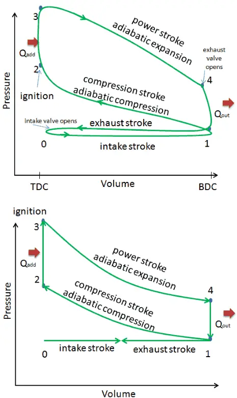
• Closed cycle. The largest difference between the two diagrams is the simplification of the intake and exhaust strokes in the ideal cycle. In the exhaust stroke, heat Q_out is ejected to the environment, in a real engine, the gas leaves the engine and is replaced by a new mixture of air and fuel.
• Instantaneous heat addition (isochoric heat addition). In real engines the heat addition is not instantaneous, therefore the peak pressure is not at TDC, but just after TDC.
• No heat transfer (adiabatic)
  • Compression – The gas (fuel-air mixture) is compressed adiabatically from state 1 to state 2. In real engines, there are always some inefficiencies that reduce the thermal efficiency.
  • Expansion. The gas (fuel-air mixture) expands adiabatically from state 3 to state 4.
• Complete combustion of fuel-air mixture.
• No pumping work. Pumping work is the difference between the work done during exhaust stroke and the work done during intake stroke. In real cycles, there is a pressure difference between exhaust and inlet pressures.
• No blowdown loss. Blowdown loss is caused by the early opening of exhaust valves. This results in a loss of work output during expansion stroke.
• No blow-by loss. The blow-by loss is caused by the leakage of compressed gases through piston rings and other crevices.
• No frictional losses.

These simplifying assumptions and losses lead to the fact that the enclosed area (work) of the pV diagram for an actual engine is significantly smaller than the size of the area (work) enclosed by the pV diagram of the ideal cycle. In other words, the ideal engine cycle will overestimate the net work and, if the engines run at the same speed, greater power produced by the actual engine by around 20%.

See also:

Otto Cycle