Calculation of Thermal Efficiency
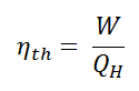
As a result of this statement, we define the thermal efficiency, ηth, of any heat engine as the ratio of the work it does, W, to the heat input at the high temperature, QH.
The thermal efficiency, ηth, represents the fraction of heat, QH, that is converted to work. It is a dimensionless performance measure of a heat engine that uses thermal energy, such as a steam turbine, an internal combustion engine, or a refrigerator. For a refrigeration or heat pumps, thermal efficiency indicates the extent to which the energy added by work is converted to net heat output. Since it is dimensionless number, we must always express W, QH, and QC in the same units.
Since energy is conserved according to the first law of thermodynamics and energy cannot be be converted to work completely, the heat input, QH, must equal the work done, W, plus the heat that must be dissipated as waste heat QC into the environment. Therefore we can rewrite the formula for thermal efficiency as:
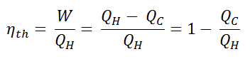
To give the efficiency as a percent, we multiply the previous formula by 100. Note that, ηth could be 100% only if the waste heat QC will be zero.
In general, the efficiency of even the best heat engines is quite low. In short, it is very difficult to convert thermal energy to mechanical energy. The thermal efficiencies are usually below 50% and often far below. Be careful when you compare it with efficiencies of wind or hydro power (wind turbines are not heat engines), there is no energy conversion between the thermal and mechanical energy.
Calculation of Brayton Cycle
Let assume the ideal Brayton cycle that describes the workings of a constant pressure heat engine. Modern gas turbine engines and airbreathing jet engines also follow the Brayton cycle. This cycle consist of four thermodynamic processes:
-
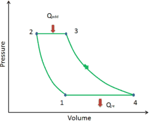
Ideal Brayton cycle consist of four thermodynamic processes. Two isentropic processes and two isobaric processes. isentropic compression – ambient air is drawn into the compressor, where it is pressurized (1 → 2). The work required for the compressor is given by WC = H2 – H1.
- isobaric heat addition – the compressed air then runs through a combustion chamber, where fuel is burned and air or another medium is heated (2 → 3). It is a constant-pressure process, since the chamber is open to flow in and out. The net heat added is given by Qadd = H3 – H2
- isentropic expansion – the heated, pressurized air then expands on turbine, gives up its energy. The work done by turbine is given by WT = H4 – H3
- isobaric heat rejection – the residual heat must be rejected in order to close the cycle. The net heat rejected is given by Qre = H4 – H1
As can be seen, we can describe and calculate (e.g. thermodynamic efficiency) such cycles (similarly for Rankine cycle) using enthalpies.
To calculate the thermal efficiency of the Brayton cycle (single compressor and single turbine) engineers use the first law of thermodynamics in terms of enthalpy rather than in terms of internal energy.
The first law in terms of enthalpy is:
dH = dQ + Vdp
In this equation the term Vdp is a flow process work. This work, Vdp, is used for open flow systems like a turbine or a pump in which there is a “dp”, i.e. change in pressure. There are no changes in control volume. As can be seen, this form of the law simplifies the description of energy transfer.
There are expressions in terms of more familiar variables such as temperature and pressure:
dH = CpdT + V(1-αT)dp
Where Cp is the heat capacity at constant pressure and α is the coefficient of (cubic) thermal expansion. For ideal gas αT = 1 and therefore:
dH = CpdT
At constant pressure, the enthalpy change equals the energy transferred from the environment through heating:
Isobaric process (Vdp = 0):
dH = dQ → Q = H2 – H1 → H2 – H1 = Cp (T2 – T1)
At constant entropy, i.e. in isentropic process, the enthalpy change equals the flow process work done on or by the system:
Isentropic process (dQ = 0):
dH = Vdp → W = H2 – H1 → H2 – H1 = Cp (T2 – T1)

The enthalpy can be made into an intensive, or specific, variable by dividing by the mass. Engineers use the specific enthalpy in thermodynamic analysis more than the enthalpy itself. The thermal efficiency of such simple Brayton cycle, for ideal gas and in terms of specific enthalpies can now be expressed in terms of the temperatures:

Calculation of Rankine Cycle

The Rankine cycle closely describes the processes in steam-operated heat engines commonly found in most of thermal power plants. The heat sources used in these power plants are usually the combustion of fossil fuels such as coal, natural gas, or also the nuclear fission.
A nuclear power plant (nuclear power station) looks like a standard thermal power station with one exception. The heat source in the nuclear power plant is a nuclear reactor. As is typical in all conventional thermal power stations the heat is used to generate steam which drives a steam turbine connected to a generator which produces electricity.
Typically most of nuclear power plants operates multi-stage condensing steam turbines. In these turbines the high-pressure stage receives steam (this steam is nearly saturated steam – x = 0.995 – point C at the figure; 6 MPa; 275.6°C) from a steam generator and exhaust it to moisture separator-reheater (point D). The steam must be reheated in order to avoid damages that could be caused to blades of steam turbine by low quality steam. The reheater heats the steam (point D) and then the steam is directed to the low-pressure stage of steam turbine, where expands (point E to F). The exhausted steam then condenses in the condenser and it is at a pressure well below atmospheric (absolute pressure of 0.008 MPa), and is in a partially condensed state (point F), typically of a quality near 90%.
In this case, steam generators, steam turbine, condensers and feedwater pumps constitute a heat engine, that is subject to the efficiency limitations imposed by the second law of thermodynamics. In ideal case (no friction, reversible processes, perfect design), this heat engine would have a Carnot efficiency of
= 1 – Tcold/Thot = 1 – 315/549 = 42.6%
where the temperature of the hot reservoir is 275.6°C (548.7K), the temperature of the cold reservoir is 41.5°C (314.7K). But the nuclear power plant is the real heat engine, in which thermodynamic processes are somehow irreversible. They are not done infinitely slowly. In real devices (such as turbines, pumps, and compressors) a mechanical friction and heat losses cause further efficiency losses.
To calculate the thermal efficiency of the simplest Rankine cycle (without reheating) engineers use the first law of thermodynamics in terms of enthalpy rather than in terms of internal energy.
The first law in terms of enthalpy is:
dH = dQ + Vdp
In this equation the term Vdp is a flow process work. This work, Vdp, is used for open flow systems like a turbine or a pump in which there is a “dp”, i.e. change in pressure. There are no changes in control volume. As can be seen, this form of the law simplifies the description of energy transfer. At constant pressure, the enthalpy change equals the energy transferred from the environment through heating:
Isobaric process (Vdp = 0):
dH = dQ → Q = H2 – H1
At constant entropy, i.e. in isentropic process, the enthalpy change equals the flow process work done on or by the system:
Isentropic process (dQ = 0):
dH = Vdp → W = H2 – H1
It is obvious, it will be very useful in analysis of both thermodynamic cycles used in power engineering, i.e. in Brayton cycle and Rankine cycle.
The enthalpy can be made into an intensive, or specific, variable by dividing by the mass. Engineers use the specific enthalpy in thermodynamic analysis more than the enthalpy itself. It is tabulated in the steam tables along with specific volume and specific internal energy. The thermal efficiency of such simple Rankine cycle and in terms of specific enthalpies would be:
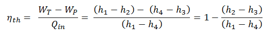
It is very simple equation and for determination of the thermal efficiency you can use data from steam tables.
In modern nuclear power plants the overall thermal efficiency is about one-third (33%), so 3000 MWth of thermal power from the fission reaction is needed to generate 1000 MWe of electrical power. The reason lies in relatively low steam temperature (6 MPa; 275.6°C). Higher efficiencies can be attained by increasing the temperature of the steam. But this requires an increase in pressures inside boilers or steam generators. However, metallurgical considerations place an upper limits on such pressures. In comparison to other energy sources the thermal efficiency of 33% is not much. But it must be noted that nuclear power plants are much more complex than fossil fuel power plants and it is much easier to burn fossil fuel ,than to generate energy from nuclear fuel. Sub-critical fossil fuel power plants, that are operated under critical pressure (i.e. lower than 22.1 MPa), can achieve 36–40% efficiency.
We hope, this article, Calculation of Thermal Efficiency, helps you. If so, give us a like in the sidebar. Main purpose of this website is to help the public to learn some interesting and important information about thermal engineering.