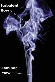
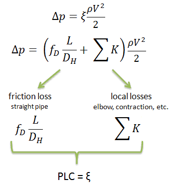
Characteristics of turbulent flow. Turbulent flow tends to occur at higher velocities, low viscosity and at higher characteristic linear dimensions. Thermal Engineering
Characteristics of Turbulent Flow
- Turbulent flow tends to occur at higher velocities, low viscosity and at higher characteristic linear dimensions.
- If the Reynolds number is greater than Re > 3500, the flow is turbulent.
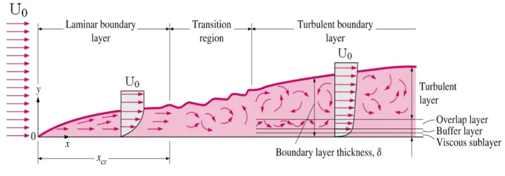
- Irregularity: The flow is characterized by the irregular movement of particles of the fluid. The movement of fluid particles is chaotic. For this reason, turbulent flow is normally treated statistically rather than deterministically.
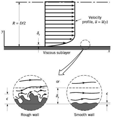
- Diffusivity: In turbulent flow, a fairly flat velocity distribution exists across the section of pipe, with the result that the entire fluid flows at a given single value and drops rapidly extremely close to the walls. The characteristic which is responsible for the enhanced mixing and increased rates of mass, momentum and energy transports in a flow is called “diffusivity”.
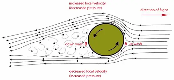
- Rotationality: Turbulent flow is characterized by a strong three-dimensional vortex generation mechanism. This mechanism is known as vortex stretching.
- Dissipation: A dissipative process is a process in which the kinetic energy of turbulent flow is transformed into internal energy by viscous shear stress.
Source: Blevins, R. D. (1990), Flow Induced Vibration, 2nd Edn., Van Nostrand Reinhold Co.
Laminar vs. Turbulent Flow
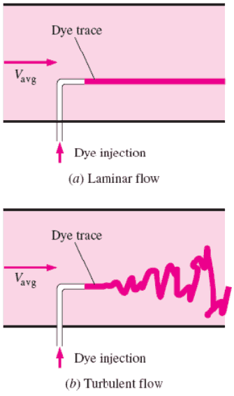
- Re < 2000
- ‘low’ velocity
- Fluid particles move in straight lines
- Layers of water flow over one another at different speeds with virtually no mixing between layers.
- The flow velocity profile for laminar flow in circular pipes is parabolic in shape, with a maximum flow in the center of the pipe and a minimum flow at the pipe walls.
- The average flow velocity is approximately one half of the maximum velocity.
- Simple mathematical analysis is possible.
- Rare in practice in water systems.
- Re > 4000
- ‘high’ velocity
- The flow is characterized by the irregular movement of particles of the fluid.
- Average motion is in the direction of the flow
- The flow velocity profile for turbulent flow is fairly flat across the center section of a pipe and drops rapidly extremely close to the walls.
- The average flow velocity is approximately equal to the velocity at the center of the pipe.
- Mathematical analysis is very difficult.
- Most common type of flow.
We hope, this article, Characteristics of Turbulent Flow, helps you. If so, give us a like in the sidebar. Main purpose of this website is to help the public to learn some interesting and important information about thermal engineering.