Thermal Engineering

Bernoulli’s Equation

The Bernoulli’s equation can be considered to be a statement of the conservation of energy principle appropriate for flowing fluids. It is one of the most important/useful equations in fluid mechanics. It puts into a relation pressure and velocity in an inviscid incompressible flow. Bernoulli’s equation has some restrictions in its applicability, they summarized in following points:

• steady flow system,
• density is constant (which also means the fluid is incompressible),
• no work is done on or by the fluid,
• no heat is transferred to or from the fluid,
• no change occurs in the internal energy,
• the equation relates the states at two points along a single streamline (not conditions on two different streamlines)

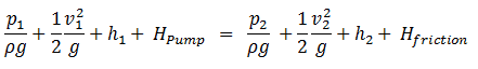
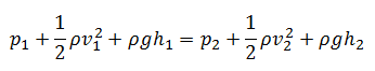
Under these conditions, the general energy equation is simplified to:

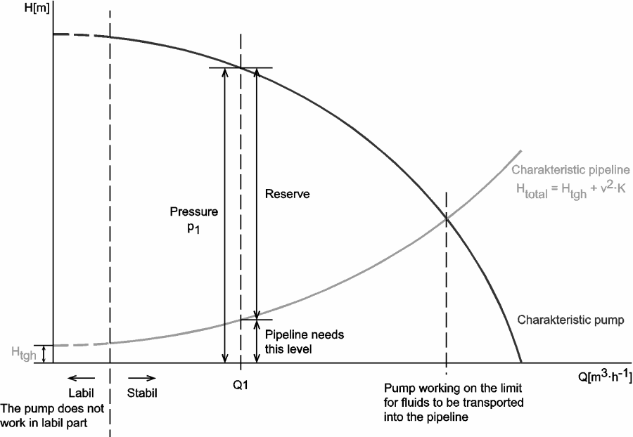
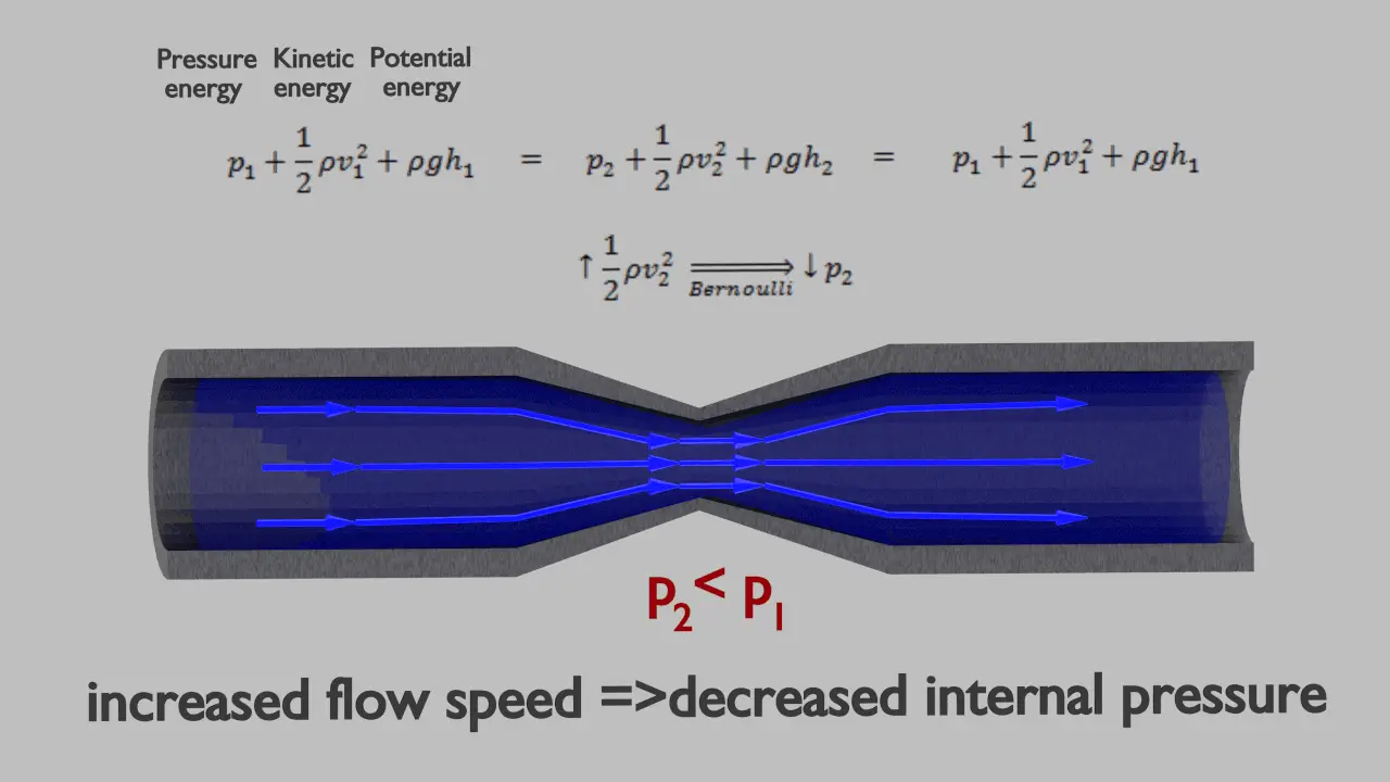
This equation is the most famous equation in fluid dynamics. The Bernoulli’s equation describes the qualitative behavior flowing fluid that is usually labeled with the term Bernoulli’s effect. This effect causes the lowering of fluid pressure in regions where the flow velocity is increased. This lowering of pressure in a constriction of a flow path may seem counterintuitive, but seems less so when you consider pressure to be energy density. In the high velocity flow through the constriction, kinetic energy must increase at the expense of pressure energy. The dimensions of terms in the equation are kinetic energy per unit volume.

Bernoulli’s Effect – Relation between Pressure and Velocity

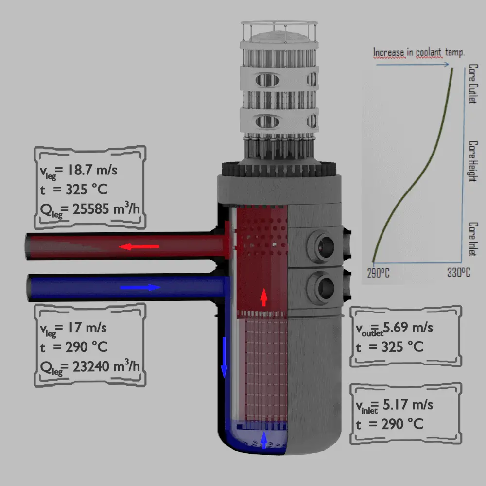
It is an illustrative example, following data do not correspond to any reactor design.

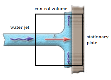
When the Bernoulli’s equation is combined with the continuity equation the two can be used to find velocities and pressures at points in the flow connected by a streamline.

The continuity equation is simply a mathematical expression of the principle of conservation of mass. For a control volume that has a single inlet and a single outlet, the principle of conservation of mass states that, for steady-state flow, the mass flow rate into the volume must equal the mass flow rate out.

Example:

Determine pressure and velocity within a cold leg of primary piping and determine pressure and velocity at a bottom of a reactor core, which is about 5 meters below the cold leg of primary piping.

Let assume:

• Fluid of constant density ⍴ ~ 720 kg/m³ (at 290°C) is flowing steadily through the cold leg and through the core bottom.

• Primary piping flow cross-section (single loop) is equal to 0.385 m² (piping diameter ~ 700mm)

• Flow velocity in the cold leg is equal to 17 m/s.

• Reactor core flow cross-section is equal to 5m².

• The gauge pressure inside the cold leg is equal to 16 MPa.

As a result of the Continuity principle the velocity at the bottom of the core is:

v_inlet =  v_cold . A_piping / A_core = 17 x 1.52 / 5 = 5.17 m/s

As a result of the Bernoulli’s principle the pressure at the bottom of the core (core inlet) is:

 

See also:

Bernoulli’s Principle

Extended Bernoulli’s Equation

There are two main assumptions, that were applied on the derivation of the simplified Bernoulli’s equation.

• The first restriction on Bernoulli’s equation is that no work is allowed to be done on or by the fluid. This is a significant limitation, because most hydraulic systems (especially in nuclear engineering) include pumps. This restriction prevents two points in a fluid stream from being analyzed if a pump exists between the two points.

• The second restriction on simplified Bernoulli’s equation is that no fluid friction is allowed in solving hydraulic problems. In reality, friction plays crucial role. The total head possessed by the fluid cannot be transferred completely and lossless from one point to another. In reality, one purpose of pumps incorporated in a hydraulic system is to overcome the losses in pressure due to friction.

Due to these restrictions most of practical applications of the simplified Bernoulli’s equation to real hydraulic systems are very limited. In order to deal with both head losses and pump work, the simplified Bernoulli’s equation must be modified.

The Bernoulli equation can be modified to take into account gains and losses of head. The resulting equation, referred to as the extended Bernoulli’s equation, is very useful in solving most fluid flow problems. The following equation is one form of the extended Bernoulli’s equation.

where:
h = height above reference level (m)
v = average velocity of fluid (m/s)
p = pressure of fluid (Pa)
H_pump = head added by pump (m)
H_friction = head loss due to fluid friction (m)
g = acceleration due to gravity (m/s²)

The head loss (or the pressure loss) due to fluid friction (H_friction) represents the energy used in overcoming friction caused by the walls of the pipe. The head loss that occurs in pipes is dependent on the flow velocity, pipe diameter and length, and a friction factor based on the roughness of the pipe and the Reynolds number of the flow. A piping system containing many pipe fittings and joints, tube convergence, divergence, turns, surface roughness and other physical properties will also increase the head loss of a hydraulic system.

Although the head loss represents a loss of energy, it does does not represent a loss of total energy of the fluid. The total energy of the fluid conserves as a consequence of the law of conservation of energy. In reality, the head loss due to friction results in an equivalent increase in the internal energy (increase in temperature) of the fluid.

Most methods for evaluating head loss due to friction are based almost exclusively on experimental evidence. This will be discussed in following sections.

 

 

See also:

Bernoulli’s Principle

Hydraulic Head

In general, the hydraulic head, or total head, is a measure of the potential of fluid at the measurement point. It can be used to determine a hydraulic gradient between two or more points.

In fluid dynamics, head is a concept that relates the energy in an incompressible fluid to the height of an equivalent static column of that fluid. The units for all the different forms of energy in the Bernoulli’s equation can be measured also in units of distance, and therefore these terms are sometimes referred to as “heads” (pressure head, velocity head, and elevation head). Head is also defined for pumps. This head is usually referred to as the static head and represents the maximum height (pressure) it can deliver. Therefore the characteristics of all pumps can be usually read from its Q-H curve (flow rate – height).

There are four types of potential (head):

• Pressure potential – Pressure head: The pressure head represents the flow energy of a column of fluid whose weight is equivalent to the pressure of the fluid.ρ_w: density of water assumed to be independent of pressure
• Elevation potential – Elevation head: The elevation head represents the potential energy of a fluid due to its elevation above a reference level.
• Kinetic potential – Kinetic head: The kinetic head represents the kinetic energy of the fluid. It is the height in feet that a flowing fluid would rise in a column if all of its kinetic energy were converted to potential energy.

The sum of the elevation head, kinetic head, and pressure head of a fluid is called the total head. Thus, Bernoulli’s equation states that the total head of the fluid is constant.

  Consider a pipe containing an ideal fluid. If this pipe undergoes a gradual expansion in diameter, the continuity equation tells us that as the pipe diameter increases, the flow velocity must decrease in order to maintain the same mass flow rate. Since the outlet velocity is less than the inlet velocity, the kinetic head of the flow must decrease from the inlet to the outlet. If there is no change in elevation head (the pipe lies horizontal), the decrease in kinetic head must be compensated for by an increase in pressure head.

 

 

See also:

Bernoulli’s Principle

Pressure Head

In general, the hydraulic head, or total head, is a measure of the potential of fluid at the measurement point. It can be used to determine a hydraulic gradient between two or more points.

In fluid dynamics, head is a concept that relates the energy in an incompressible fluid to the height of an equivalent static column of that fluid. The units for all the different forms of energy in the Bernoulli’s equation can be measured also in units of distance, and therefore these terms are sometimes referred to as “heads” (pressure head, velocity head, and elevation head). Head is also defined for pumps. This head is usually referred to as the static head and represents the maximum height (pressure) it can deliver. Therefore the characteristics of all pumps can be usually read from its Q-H curve (flow rate – height).

There are four types of potential (head):

• Pressure potential – Pressure head: The pressure head represents the flow energy of a column of fluid whose weight is equivalent to the pressure of the fluid.ρ_w: density of water assumed to be independent of pressure
• Elevation potential – Elevation head: The elevation head represents the potential energy of a fluid due to its elevation above a reference level.
• Kinetic potential – Kinetic head: The kinetic head represents the kinetic energy of the fluid. It is the height in feet that a flowing fluid would rise in a column if all of its kinetic energy were converted to potential energy.

The sum of the elevation head, kinetic head, and pressure head of a fluid is called the total head. Thus, Bernoulli’s equation states that the total head of the fluid is constant.

  Consider a pipe containing an ideal fluid. If this pipe undergoes a gradual expansion in diameter, the continuity equation tells us that as the pipe diameter increases, the flow velocity must decrease in order to maintain the same mass flow rate. Since the outlet velocity is less than the inlet velocity, the kinetic head of the flow must decrease from the inlet to the outlet. If there is no change in elevation head (the pipe lies horizontal), the decrease in kinetic head must be compensated for by an increase in pressure head.

 

 

See also:

Bernoulli’s Principle

Velocity Head

In general, the hydraulic head, or total head, is a measure of the potential of fluid at the measurement point. It can be used to determine a hydraulic gradient between two or more points.

In fluid dynamics, head is a concept that relates the energy in an incompressible fluid to the height of an equivalent static column of that fluid. The units for all the different forms of energy in the Bernoulli’s equation can be measured also in units of distance, and therefore these terms are sometimes referred to as “heads” (pressure head, velocity head, and elevation head). Head is also defined for pumps. This head is usually referred to as the static head and represents the maximum height (pressure) it can deliver. Therefore the characteristics of all pumps can be usually read from its Q-H curve (flow rate – height).

There are four types of potential (head):

• Pressure potential – Pressure head: The pressure head represents the flow energy of a column of fluid whose weight is equivalent to the pressure of the fluid.ρ_w: density of water assumed to be independent of pressure
• Elevation potential – Elevation head: The elevation head represents the potential energy of a fluid due to its elevation above a reference level.
• Kinetic potential – Kinetic head: The kinetic head represents the kinetic energy of the fluid. It is the height in feet that a flowing fluid would rise in a column if all of its kinetic energy were converted to potential energy.

The sum of the elevation head, kinetic head, and pressure head of a fluid is called the total head. Thus, Bernoulli’s equation states that the total head of the fluid is constant.

  Consider a pipe containing an ideal fluid. If this pipe undergoes a gradual expansion in diameter, the continuity equation tells us that as the pipe diameter increases, the flow velocity must decrease in order to maintain the same mass flow rate. Since the outlet velocity is less than the inlet velocity, the kinetic head of the flow must decrease from the inlet to the outlet. If there is no change in elevation head (the pipe lies horizontal), the decrease in kinetic head must be compensated for by an increase in pressure head.

 

 

See also:

Bernoulli’s Principle

Elevation Head

In general, the hydraulic head, or total head, is a measure of the potential of fluid at the measurement point. It can be used to determine a hydraulic gradient between two or more points.

In fluid dynamics, head is a concept that relates the energy in an incompressible fluid to the height of an equivalent static column of that fluid. The units for all the different forms of energy in the Bernoulli’s equation can be measured also in units of distance, and therefore these terms are sometimes referred to as “heads” (pressure head, velocity head, and elevation head). Head is also defined for pumps. This head is usually referred to as the static head and represents the maximum height (pressure) it can deliver. Therefore the characteristics of all pumps can be usually read from its Q-H curve (flow rate – height).

There are four types of potential (head):

• Pressure potential – Pressure head: The pressure head represents the flow energy of a column of fluid whose weight is equivalent to the pressure of the fluid.ρ_w: density of water assumed to be independent of pressure
• Elevation potential – Elevation head: The elevation head represents the potential energy of a fluid due to its elevation above a reference level.
• Kinetic potential – Kinetic head: The kinetic head represents the kinetic energy of the fluid. It is the height in feet that a flowing fluid would rise in a column if all of its kinetic energy were converted to potential energy.

The sum of the elevation head, kinetic head, and pressure head of a fluid is called the total head. Thus, Bernoulli’s equation states that the total head of the fluid is constant.

  Consider a pipe containing an ideal fluid. If this pipe undergoes a gradual expansion in diameter, the continuity equation tells us that as the pipe diameter increases, the flow velocity must decrease in order to maintain the same mass flow rate. Since the outlet velocity is less than the inlet velocity, the kinetic head of the flow must decrease from the inlet to the outlet. If there is no change in elevation head (the pipe lies horizontal), the decrease in kinetic head must be compensated for by an increase in pressure head.

 

 

See also:

Bernoulli’s Principle

Head Loss – Pressure Loss

In the practical analysis of piping systems the quantity of most importance is the pressure loss due to viscous effects along the length of the system, as well as additional pressure losses arising from other technological equipments like, valves, elbows, piping entrances, fittings and tees.
At first, an extended Bernoulli’s equation must be introduced. This equation permits account of viscosity to be included in an empirical way and quantify this with a physical parameter known as the head loss.

The head loss (or the pressure loss) represents the reduction in the total head or pressure (sum of elevation head, velocity head and pressure head) of the fluid as it flows through a hydraulic system. The head loss also represents the energy used in overcoming friction caused by the walls of the pipe and other technological equipments. The head loss is unavoidable in real moving fluids. It is present because of the friction between adjacent fluid particles as they move relative to one another (especially in turbulent flow).

The head loss that occurs in pipes is dependent on the flow velocity, pipe diameter and length, and a friction factor based on the roughness of the pipe and the Reynolds number of the flow. Although the head loss represents a loss of energy, it does not represent a loss of total energy of the fluid. The total energy of the fluid conserves as a consequence of the law of conservation of energy. In reality, the head loss due to friction results in an equivalent increase in the internal energy (increase in temperature) of the fluid.

Most methods for evaluating head loss due to friction are based almost exclusively on experimental evidence. This will be discussed in following sections.

Classification of Head Loss

The head loss of a pipe, tube or duct system, is the same as that produced in a straight pipe or duct whose length is equal to the pipes of the original systems plus the sum of the equivalent lengths of all the components in the system.

As can be seen, the head loss of piping system is divided into two main categories, “major losses” associated with energy loss per length of pipe, and “minor losses” associated with bends, fittings, valves, etc.

• Major Head Loss – due to friction in pipes and ducts.
• Minor Head Loss – due to components as valves, fittings, bends and tees.

The head loss can be then expressed as:

h_loss = Σ h_{major_losses} + Σ h_{minor_losses}

Summary:

• Head loss or pressure loss are the reduction in the total head (sum of potential head, velocity head, and pressure head) of a fluid caused by the friction present in the fluid’s motion.
• Head loss and pressure loss represent the same phenomenon – frictional losses in pipe and losses in hydraulic components, but they are expressed in different units.
• Head loss of hydraulic system is divided into two main categories:
  • Major Head Loss – due to friction in straight pipes
  • Minor Head Loss – due to components as valves, bends…
• Darcy’s equation can be used to calculate major losses.
• A special form of Darcy’s equation can be used to calculate minor losses.
• The friction factor for fluid flow can be determined using a Moody chart.

Why the head loss is very important?

As can be seen from the picture, the head loss is forms key characteristic of any hydraulic system. In systems, in which some certain flowrate must be maintained (e.g. to provide sufficient cooling or heat transfer from a reactor core), the equilibrium of the head loss and the head added by a pump determines the flowrate through the system.

Major Head Loss – Frictional Loss

See also: Major Head Loss – Frictional Losses

Major losses, which are associated with frictional energy loss per length of pipe depends on the flow velocity, pipe length, pipe diameter, and a friction factor based on the roughness of the pipe, and whether the flow is laminar or turbulent (i.e. the Reynolds number of the flow).

Although the head loss represents a loss of energy, it does not represent a loss of total energy of the fluid. The total energy of the fluid conserves as a consequence of the law of conservation of energy. In reality, the head loss due to friction results in an equivalent increase in the internal energy (increase in temperature) of the fluid.

By observation, the major head loss is roughly proportional to the square of the flow rate in most engineering flows (fully developed, turbulent pipe flow).

The most common equation used to calculate major head losses in a tube or duct is the Darcy–Weisbach equation (head loss form).

where:

• Δh = the head loss due to friction (m)
• f_D = the Darcy friction factor (unitless)
• L = the pipe length (m)
• D = the hydraulic diameter of the pipe D (m)
• g = the gravitational constant (m/s²)
• V = the mean flow velocity V (m/s)

  Evaluating the Darcy-Weisbach equation provides insight into factors affecting the head loss in a pipeline.

• Consider that the length of the pipe or channel is doubled, the resulting frictional head loss will double.
• At constant flow rate and pipe length, the head loss is inversely proportional to the 4th power of diameter (for laminar flow), and thus reducing the pipe diameter by half increases the head loss by a factor of 16. This is a very significant increase in head loss, and shows why larger diameter pipes lead to much smaller pumping power requirements.
• Since the head loss is roughly proportional to the square of the flow rate, then if the flow rate is doubled, the head loss increases by a factor of four.
• The head loss is reduced by half (for laminar flow) when the viscosity of the fluid is reduced by half.

With the exception of the Darcy friction factor, each of these terms (the flow velocity, the hydraulic diameter, the length of a pipe) can be easily measured. The Darcy friction factor takes the fluid properties of density and viscosity into account, along with the pipe roughness. This factor may be evaluated by the use of various empirical relations, or it may be read from published charts (e.g. Moody chart).

 

Minor Head Loss – Local Pressure Loss

See also: Minor Head Loss – Local Pressure Loss

In industry any pipe system contains different technological elements as bends, fittings, valves or heated channels. These additional components add to the overall head loss of the system. Such losses are generally termed minor losses, although they often account for a major portion of the head loss. For relatively short pipe systems, with a relatively large number of bends and fittings, minor losses can easily exceed major losses (especially with a partially closed valve that can cause a greater pressure loss than a long pipe, in fact when a valve is closed or nearly closed, the minor loss is infinite).

The minor losses are commonly measured experimentally. The data, especially for valves, are somewhat dependent upon the particular manufacturer’s design.

Generally, most of methods that are used in industry, define a coefficient K as a value for certain technological component.

Like pipe friction, the minor losses are roughly proportional to the square of the flow rate and therefore they can be easy integrated into the Darcy-Weisbach equation. K is the sum of all of the loss coefficients in the length of pipe, each contributing to the overall head loss.

The following methods are of practical importance in local pressure loss calculations:

• Equivalent Length Method
• K-Method – Resistance Coefficient Method
• 2K-Method
• 3K-Method

See also: Minor Head Loss – Local Pressure Loss

 

 

Head Loss of Two-phase Fluid Flow

See also: Two-phase Pressure Drop

In contrast to single-phase pressure drops, calculation and prediction of two-phase pressure drops is much more sophisticated problem and leading methods differ significantly. Experimental data indicates that the frictional pressure drop in the two-phase flow (e.g. in a boiling channel) is substantially higher than that for a single-phase flow with the same length and mass flow rate. Explanations for this include an apparent increased surface roughness due to bubble formation on the heated surface and increased flow velocities.

 

See also:

Bernoulli’s Principle

Conservation of Momentum in Fluid Dynamics

In general, the law of conservation of momentum or principle of momentum conservation states that the momentum of an isolated system is a constant. The vector sum of the momenta (momentum is equal to the mass of an object multiplied by its velocity) of all the objects of a system cannot be changed by interactions within the system. In classical mechanics, this law is implied by Newton’s laws.

In fluid dynamics, the analysis of motion is performed in the same way as in solid mechanics – by use of Newton’s laws of motion. As can be seen moving fluids are exerting forces. The lift force on an aircraft is exerted by the air moving over the wing.

A jet of water from a hose exerts a force on whatever it hits. But here it is not clear what mass of moving fluid we should use and therefore it is necessary to use a different form of the equation.

Newton’s 2nd Law can be written:

We assume fluid to be both steady and incompressible. To determine the rate of change of momentum for a fluid we will consider a streamtube (control volume) as we did for the Bernoulli equation. In this control volume any change in momentum of the fluid within a control volume is due to the action of external forces on the fluid within the volume.

As can be seen from the picture the control volume method can be used to analyze the law of conservation of momentum in fluid. Control volume is an imaginary surface enclosing a volume of interest. The control volume can be fixed or moving, and it can be rigid or deformable. In order to determine all forces acting on the surfaces of the control volume we have to solve the conservation laws in this control volume.

The first conservation equation we have to consider in the control volume is the continuity equation (the law of conservation of matter). In the simplest form it is represented by following equation:

∑ṁ_in = ∑ṁ_out

Sum of mass flow rates entering per unit time = Sum of mass flow rates leaving per unit time

The second conservation equation we have to consider in the control volume is the momentum formula.

Momentum Formula

In the simplest form the momentum formula can be represented by following equation:

–

Choosing a Control Volume

A control volume can be selected as any arbitrary volume through which fluid flows. This volume can be static, moving, and even deforming during flow. In order to solve any problem we have to solve basic conservation laws in this volume. It is very important to know all relative flow velocities to the control surface and therefore it is very important to define exactly the boundaries of the control volume during an analysis.

Example: The force acting on a deflector elbow

An elbow (let say of primary piping) is used to deflect water flow at a velocity of 17 m/s. The piping diameter is equal to 700 mm. The gauge pressure inside the pipe is about 16 MPa at the temperature of 290°C. Fluid is of constant density ⍴ ~ 720 kg/m³ (at 290°C). The angle of the elbow is 45°.

Calculate the force on the wall of a deflector elbow (i.e. calculate vector F₃).

Assumptions:

• The flow is steady.
• The frictional losses are negligible.
• The weight of the elbow is negligible.
• The weight of the water in the elbow is negligible.

We take the elbow as the control volume. The control volume is shown at the picture. The momentum equation is a vector equation so it has three components. We take the x- and z- coordinates as shown and we will solve the problem separately according to these coordinates.

First, let us consider the component in the x-coordinate. The conservation of linear momentum equation becomes:

Second, let us consider the component in the y-coordinate. The conservation of linear momentum equation becomes:

The final force acting on the wall of a deflector elbow will be:

Example: Water Jet Striking a Stationary Plate

A stationary plate (e.g. blade of a watermill) is used to deflect water flow at a velocity of 1 m/s and at an angle of 90°. It occurs at atmospheric pressure and the mass flow rate is equal to Q =1 m³/s.

1. Calculate the pressure force.
2. Calculate the body force.
3. Calculate the total force.
4. Calculate the resultant force.

Solution

1. The pressure force is zero as the pressure at both the inlet and the outlets to the control volume are atmospheric.
2. As the control volume is small we can ignore the body force due to the weight of gravity.
3. F_x = ρ.Q.(w_1x – w_2x) = 1000 . 1 . (1 – 0) = 1000 N
   F_y = 0
   F = (1000, 0)
4. The resultant force on the plane is the same magnitude but in the opposite direction as the total force F (friction and weight are neglected).

The water jet exerts on the plate the force of 1000 N in the x-direction.

 

See also:

Fluid Dynamics

Momentum Formula – Momentum Equation

We assume fluid to be both steady and incompressible. To determine the rate of change of momentum for a fluid we will consider a streamtube (control volume) as we did for the Bernoulli equation. In this control volume any change in momentum of the fluid within a control volume is due to the action of external forces on the fluid within the volume.

As can be seen from the picture the control volume method can be used to analyze the law of conservation of momentum in fluid. Control volume is an imaginary surface enclosing a volume of interest. The control volume can be fixed or moving, and it can be rigid or deformable. In order to determine all forces acting on the surfaces of the control volume we have to solve the conservation laws in this control volume.

The first conservation equation we have to consider in the control volume is the continuity equation (the law of conservation of matter). In the simplest form it is represented by following equation:

∑ṁ_in = ∑ṁ_out

Sum of mass flow rates entering per unit time = Sum of mass flow rates leaving per unit time

The second conservation equation we have to consider in the control volume is the momentum formula.In the simplest form the momentum formula can be represented by following equation:

–

Choosing a Control Volume

A control volume can be selected as any arbitrary volume through which fluid flows. This volume can be static, moving, and even deforming during flow. In order to solve any problem we have to solve basic conservation laws in this volume. It is very important to know all relative flow velocities to the control surface and therefore it is very important to define exactly the boundaries of the control volume during an analysis.

Example: The force acting on a deflector elbow

An elbow (let say of primary piping) is used to deflect water flow at a velocity of 17 m/s. The piping diameter is equal to 700 mm. The gauge pressure inside the pipe is about 16 MPa at the temperature of 290°C. Fluid is of constant density ⍴ ~ 720 kg/m³ (at 290°C). The angle of the elbow is 45°.

Calculate the force on the wall of a deflector elbow (i.e. calculate vector F₃).

Assumptions:

• The flow is steady.
• The frictional losses are negligible.
• The weight of the elbow is negligible.
• The weight of the water in the elbow is negligible.

We take the elbow as the control volume. The control volume is shown at the picture. The momentum equation is a vector equation so it has three components. We take the x- and z- coordinates as shown and we will solve the problem separately according to these coordinates.

First, let us consider the component in the x-coordinate. The conservation of linear momentum equation becomes:

Second, let us consider the component in the y-coordinate. The conservation of linear momentum equation becomes:

The final force acting on the wall of a deflector elbow will be:

Example: Water Jet Striking a Stationary Plate

A stationary plate (e.g. blade of a watermill) is used to deflect water flow at a velocity of 1 m/s and at an angle of 90°. It occurs at atmospheric pressure and the mass flow rate is equal to Q =1 m³/s.

1. Calculate the pressure force.
2. Calculate the body force.
3. Calculate the total force.
4. Calculate the resultant force.

Solution

1. The pressure force is zero as the pressure at both the inlet and the outlets to the control volume are atmospheric.
2. As the control volume is small we can ignore the body force due to the weight of gravity.
3. F_x = ρ.Q.(w_1x – w_2x) = 1000 . 1 . (1 – 0) = 1000 N
   F_y = 0
   F = (1000, 0)
4. The resultant force on the plane is the same magnitude but in the opposite direction as the total force F (friction and weight are neglected).

The water jet exerts on the plate the force of 1000 N in the x-direction.

 

See also:

Conservation of Momentum

Example: The force acting on a deflector elbow

An elbow (let say of primary piping) is used to deflect water flow at a velocity of 17 m/s. The piping diameter is equal to 700 mm. The gauge pressure inside the pipe is about 16 MPa at the temperature of 290°C. Fluid is of constant density ⍴ ~ 720 kg/m³ (at 290°C). The angle of the elbow is 45°.

Calculate the force on the wall of a deflector elbow (i.e. calculate vector F₃).

Assumptions:

• The flow is steady.
• The frictional losses are negligible.
• The weight of the elbow is negligible.
• The weight of the water in the elbow is negligible.

We take the elbow as the control volume. The control volume is shown at the picture. The momentum equation is a vector equation so it has three components. We take the x- and z- coordinates as shown and we will solve the problem separately according to these coordinates.

First, let us consider the component in the x-coordinate. The conservation of linear momentum equation becomes:

Second, let us consider the component in the y-coordinate. The conservation of linear momentum equation becomes:

The final force acting on the wall of a deflector elbow will be:

 

See also:

Conservation of Momentum

References:

Reactor Physics and Thermal Hydraulics:
1. J. R. Lamarsh, Introduction to Nuclear Reactor Theory, 2nd ed., Addison-Wesley, Reading, MA (1983).
2. J. R. Lamarsh, A. J. Baratta, Introduction to Nuclear Engineering, 3d ed., Prentice-Hall, 2001, ISBN: 0-201-82498-1.
3. W. M. Stacey, Nuclear Reactor Physics, John Wiley & Sons, 2001, ISBN: 0- 471-39127-1.
4. Glasstone, Sesonske. Nuclear Reactor Engineering: Reactor Systems Engineering, Springer; 4th edition, 1994, ISBN: 978-0412985317
5. Todreas Neil E., Kazimi Mujid S. Nuclear Systems Volume I: Thermal Hydraulic Fundamentals, Second Edition. CRC Press; 2 edition, 2012, ISBN: 978-0415802871
6. Zohuri B., McDaniel P. Thermodynamics in Nuclear Power Plant Systems. Springer; 2015, ISBN: 978-3-319-13419-2
7. Moran Michal J., Shapiro Howard N. Fundamentals of Engineering Thermodynamics, Fifth Edition, John Wiley & Sons, 2006, ISBN: 978-0-470-03037-0
8. Kleinstreuer C. Modern Fluid Dynamics. Springer, 2010, ISBN 978-1-4020-8670-0.
9. U.S. Department of Energy, THERMODYNAMICS, HEAT TRANSFER, AND FLUID FLOW. DOE Fundamentals Handbook, Volume 1, 2 and 3. June 1992.
10. White Frank M., Fluid Mechanics, McGraw-Hill Education, 7th edition, February, 2010, ISBN: 978-0077422417