Facebook Instagram Youtube Twitter

What is Example of Isochoric Process – Isochoric Heat Addition – Definition

Example of Isochoric Process – Isochoric Heat Addition. Let assume the Otto Cycle, processes 2 → 3 and 4 → 1 are isochoric processes. Thermal Engineering

Isochoric Process – Isometric Process

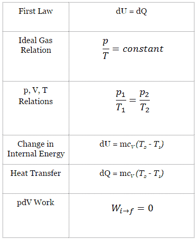
An isochoric process is a thermodynamic process, in which the volume of the closed system remains constant (V = const). It describes the behavior of gas inside the container, that cannot be deformed. Since the volume remains constant, the heat transfer into or out of the system does not the p∆V work, but only changes the internal energy (the temperature) of the system.

In engineering of internal combustion engines, isochoric processes are very important for their thermodynamic cycles (Otto and Diesel cycle), therefore the study of this process is crucial for automotive engineering.

Example of Isochoric Process – Isochoric Heat Addition
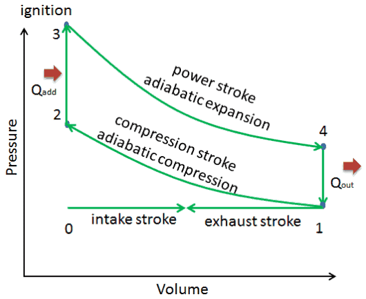
Otto Cycle - PV DiagramLet assume the Otto Cycle, which is the one of most common thermodynamic cycles that can be found in automobile engines. This cycle assumes that the heat addition occurs instantaneously (between 2 → 3) while the piston is at top dead center. This process is considered to be isochoric.

Processes 2 → 3 and 4 → 1 are isochoric processes, in which the heat is transferred into the system between 2 → 3 and out of the system between 4 → 1. During these processes no work is done on the system or extracted from the system. The isochoric process 2 → 3 is intended to represent the ignition of the fuel–air mixture and the subsequent rapid burning.
Isochoric process - main characteristics
Isochoric process – main characteristics
Guy-Lussac's Law
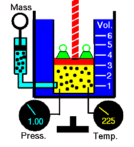
For a fixed mass of gas at constant volume, the pressure is directly proportional to the Kelvin temperature.
 
References:
Nuclear and Reactor Physics:
  1. J. R. Lamarsh, Introduction to Nuclear Reactor Theory, 2nd ed., Addison-Wesley, Reading, MA (1983).
  2. J. R. Lamarsh, A. J. Baratta, Introduction to Nuclear Engineering, 3d ed., Prentice-Hall, 2001, ISBN: 0-201-82498-1.
  3. W. M. Stacey, Nuclear Reactor Physics, John Wiley & Sons, 2001, ISBN: 0- 471-39127-1.
  4. Glasstone, Sesonske. Nuclear Reactor Engineering: Reactor Systems Engineering, Springer; 4th edition, 1994, ISBN: 978-0412985317
  5. W.S.C. Williams. Nuclear and Particle Physics. Clarendon Press; 1 edition, 1991, ISBN: 978-0198520467
  6. Kenneth S. Krane. Introductory Nuclear Physics, 3rd Edition, Wiley, 1987, ISBN: 978-0471805533
  7. G.R.Keepin. Physics of Nuclear Kinetics. Addison-Wesley Pub. Co; 1st edition, 1965
  8. Robert Reed Burn, Introduction to Nuclear Reactor Operation, 1988.
  9. U.S. Department of Energy, Nuclear Physics and Reactor Theory. DOE Fundamentals Handbook, Volume 1 and 2. January 1993.

Advanced Reactor Physics:

  1. K. O. Ott, W. A. Bezella, Introductory Nuclear Reactor Statics, American Nuclear Society, Revised edition (1989), 1989, ISBN: 0-894-48033-2.
  2. K. O. Ott, R. J. Neuhold, Introductory Nuclear Reactor Dynamics, American Nuclear Society, 1985, ISBN: 0-894-48029-4.
  3. D. L. Hetrick, Dynamics of Nuclear Reactors, American Nuclear Society, 1993, ISBN: 0-894-48453-2.
  4. E. E. Lewis, W. F. Miller, Computational Methods of Neutron Transport, American Nuclear Society, 1993, ISBN: 0-894-48452-4.

See also:

Isochoric Process

We hope, this article, Example of Isochoric Process – Isochoric Heat Addition, helps you. If so, give us a like in the sidebar. Main purpose of this website is to help the public to learn some interesting and important information about thermal engineering.
What is Polytropic Process – Definition

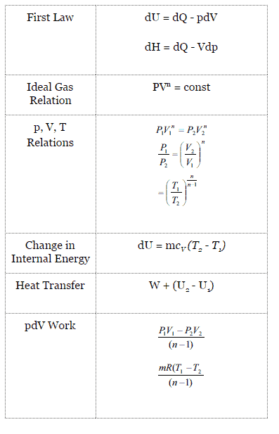
A polytropic process is any thermodynamic process that can be expressed by the following equation: pVn = constant. Definition and characteristics of Polytropic Process. Thermal Engineering

Polytropic Process

A polytropic process is any thermodynamic process that can be expressed by the following equation:

pVn = constant

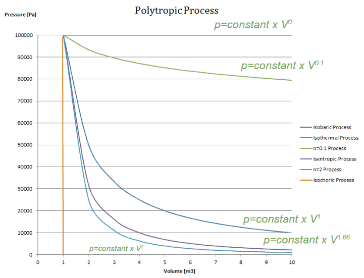
The polytropic process can describe gas expansion and compression which include heat transfer. The exponent n is known as the polytropic index and it may take on any value from 0 to ∞, depending on the particular process.

There are some special cases of n, which corresponds to particular processes:


  • the case 1 < n < , in this process heat and work flows go in opposite directions, This process occurs, for example, in vapor compression refrigeration during compression
  • the case < n < ∞, in this process heat and work flows go in the same direction, This process occurs, for example, in an internal combustion engine (e.g. Otto cycle), in which there are heat loses through the cylinder walls during gas expansion (power stroke).

For a polytropic process between two states:

p1V1n = p2V2n

Polytropic process - main characteristics
Polytropic process – main characteristics
polytropic process - pv diagram
Polytropic processes with various polytropic indexes.
 
References:
Nuclear and Reactor Physics:
  1. J. R. Lamarsh, Introduction to Nuclear Reactor Theory, 2nd ed., Addison-Wesley, Reading, MA (1983).
  2. J. R. Lamarsh, A. J. Baratta, Introduction to Nuclear Engineering, 3d ed., Prentice-Hall, 2001, ISBN: 0-201-82498-1.
  3. W. M. Stacey, Nuclear Reactor Physics, John Wiley & Sons, 2001, ISBN: 0- 471-39127-1.
  4. Glasstone, Sesonske. Nuclear Reactor Engineering: Reactor Systems Engineering, Springer; 4th edition, 1994, ISBN: 978-0412985317
  5. W.S.C. Williams. Nuclear and Particle Physics. Clarendon Press; 1 edition, 1991, ISBN: 978-0198520467
  6. Kenneth S. Krane. Introductory Nuclear Physics, 3rd Edition, Wiley, 1987, ISBN: 978-0471805533
  7. G.R.Keepin. Physics of Nuclear Kinetics. Addison-Wesley Pub. Co; 1st edition, 1965
  8. Robert Reed Burn, Introduction to Nuclear Reactor Operation, 1988.
  9. U.S. Department of Energy, Nuclear Physics and Reactor Theory. DOE Fundamentals Handbook, Volume 1 and 2. January 1993.

Advanced Reactor Physics:

  1. K. O. Ott, W. A. Bezella, Introductory Nuclear Reactor Statics, American Nuclear Society, Revised edition (1989), 1989, ISBN: 0-894-48033-2.
  2. K. O. Ott, R. J. Neuhold, Introductory Nuclear Reactor Dynamics, American Nuclear Society, 1985, ISBN: 0-894-48029-4.
  3. D. L. Hetrick, Dynamics of Nuclear Reactors, American Nuclear Society, 1993, ISBN: 0-894-48453-2.
  4. E. E. Lewis, W. F. Miller, Computational Methods of Neutron Transport, American Nuclear Society, 1993, ISBN: 0-894-48452-4.

See also:

Thermodynamic Processes

We hope, this article, Polytropic Process, helps you. If so, give us a like in the sidebar. Main purpose of this website is to help the public to learn some interesting and important information about thermal engineering.
What is Throttling Process – Isenthalpic Process – Definition

A throttling process is one of isenthalpic processes. A throttling process is a thermodynamic process, in which the enthalpy of the gas remains constant. Thermal Engineering

Throttling Process – Isenthalpic Process

A throttling process is a thermodynamic process, in which the enthalpy of the gas or medium remains constant (h = const). In fact, the throttling process is one of isenthalpic processes. During the throttling process no work is done by or on the system (dW = 0), and usually there is no heat tranfer (adiabatic) from or into the system (dQ = 0). On the other the throttling process cannot be isentropic, it is a fundamentally irreversible process. Characteristics of throttling process:

  1. No Work Transfer
  2. No Heat Transfer
  3. Irreversible Process
  4. Isenthalpic Process

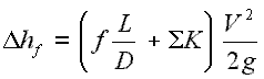
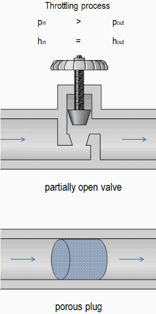
A throttling of the flow causes significant reduction in pressure, becauses a throttling device causes a local pressure loss. A throttling can be achieved simply by introducing a restriction into a line through which a gas or liquid flows. This restriction is commonly done by means of a partially open valve or a porous plug. Such pressure losses are generally termed minor losses, although they often account for a major portion of the head loss. The minor losses are roughly proportional to the square of the flow rate and therefore they can be easy integrated into the Darcy-Weisbach equation through resistance coefficient K.

minor head loss - equation

For example, consider a throttling of an ideal gas flowing through a valve that is partially open. From experience we can observe that: pin > pout, vin < vout, where p is the pressure and v is the specific volume. We can also observe that specific enthalpies remains the same, i.e. hin = hout.

The specific enthalpy is equal to the specific internal energy of the system plus the product of pressure and specific volume.

h = u + pv

Therefore, if pressure decreases then specific volume must increase if enthalpy is to remain constant (assuming u is constant). Because mass flow is constant, the change in specific volume is observed as an increase in gas velocity, and this is also verified by observations.

If there is a change in the internal energy, u, then there must be a temperature change. Normally the temperature of the fluid will drop. However in special cases, the temperature may remain the same or it may increase.

A partially open valve or a porous plug
A partially open valve or a porous plug can be used to reduce the pressure in a system.

Joule–Thomson effect – Joule Thomson coefficient

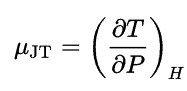
The changes of the temperature during throttling process are subject of the  Joule-Thomson effect. At room temperature and normal pressures, all gases except hydrogen and helium cool during gas expansion. The cooling occurs because work must be done to overcome the long-range attraction between the gas molecules as they move farther apart. The effect depends on the value of the Joule-Thomson coefficient, which is defined as:

Joule Thomson coefficient - equation

An application of the throttling process occurs in vapor-compression refrigerators, where a throttling valve is used to reduce the pressure and reduce the temperature of the refrigerant from the pressure at the exit of the condenser to the lower pressure existing in the evaporator.

Throttling of Wet Steam

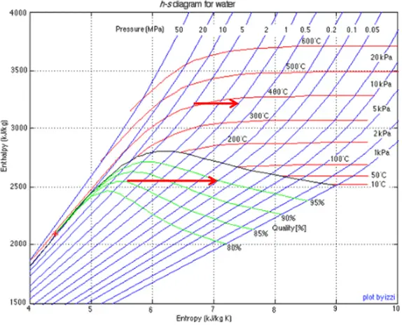
Wet steam is characterized by the vapor quality, which ranges from zero to unity – open interval (0,1).  Throttling of the wet steam is also associated with conservation of enthalpy. Enthalpy is conserved because no work is done by or on the system (dW = 0), and usually there is no heat tranfer (adiabatic) from or into the system (dQ = 0). But in this case a reduction in pressure causes an increase in vapor quality. As the pressure drops some of the liquid in the wet steam vaporizes and increases the vapor quality (i.e. dryness fraction). This process take place, because the saturation temperature is lower at the lower pressure. The lower temperature, lower pressure, higher quality steam contains the same enthalpy as the original steam.

throttling process - hs diagram - steam

Example: Throttling of Wet Steam

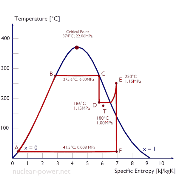
A high-pressure stage of steam turbine operates at steady state with inlet conditions of  6 MPa, t = 275.6°C, x = 1 (point C). Steam leaves this stage of turbine at a pressure of 1.15 MPa, 186°C and x = 0.87 (point D). Determine the vapor quality of the steam when throttled from 1.15 MPa to 1.0 MPa. Assume the process is adiabatic and no work is done by the system.

See also: Steam Tables

Solution:

The enthalpy for the state D must be calculated using vapor quality:

hD, wet = hD,vapor x + (1 – x ) hD,liquid  = 2782 . 0.87 + (1 – 0.87) . 790 = 2420 + 103 = 2523 kJ/kg

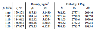
Since it is an isenthalpic process, we know the enthalpy for point T. From steam tables we have to find the vapor quality using the same equation and solving the equation for vapor quality, x:

hT, wet = hT,vapor x + (1 – x ) hT,liquid

x = (hT, wet – hT, liquid) / (hT, vapor – hT, liquid) = (2523 – 762) / (2777 – 762) = 0.874 = 87.4%

throttling process - parameters

In this case of the throttling process (1.15MPa to 1MPa) the vapor quality increases from 87% to 87.4% and the temperature decreases from 186°C to 179.9°C.

Throttling of wet steam
Throttling of wet steam usually causes an increase in vapor quality, increase in entropy and decrease in temperature.
 
References:
Nuclear and Reactor Physics:
  1. J. R. Lamarsh, Introduction to Nuclear Reactor Theory, 2nd ed., Addison-Wesley, Reading, MA (1983).
  2. J. R. Lamarsh, A. J. Baratta, Introduction to Nuclear Engineering, 3d ed., Prentice-Hall, 2001, ISBN: 0-201-82498-1.
  3. W. M. Stacey, Nuclear Reactor Physics, John Wiley & Sons, 2001, ISBN: 0- 471-39127-1.
  4. Glasstone, Sesonske. Nuclear Reactor Engineering: Reactor Systems Engineering, Springer; 4th edition, 1994, ISBN: 978-0412985317
  5. W.S.C. Williams. Nuclear and Particle Physics. Clarendon Press; 1 edition, 1991, ISBN: 978-0198520467
  6. Kenneth S. Krane. Introductory Nuclear Physics, 3rd Edition, Wiley, 1987, ISBN: 978-0471805533
  7. G.R.Keepin. Physics of Nuclear Kinetics. Addison-Wesley Pub. Co; 1st edition, 1965
  8. Robert Reed Burn, Introduction to Nuclear Reactor Operation, 1988.
  9. U.S. Department of Energy, Nuclear Physics and Reactor Theory. DOE Fundamentals Handbook, Volume 1 and 2. January 1993.

Advanced Reactor Physics:

  1. K. O. Ott, W. A. Bezella, Introductory Nuclear Reactor Statics, American Nuclear Society, Revised edition (1989), 1989, ISBN: 0-894-48033-2.
  2. K. O. Ott, R. J. Neuhold, Introductory Nuclear Reactor Dynamics, American Nuclear Society, 1985, ISBN: 0-894-48029-4.
  3. D. L. Hetrick, Dynamics of Nuclear Reactors, American Nuclear Society, 1993, ISBN: 0-894-48453-2.
  4. E. E. Lewis, W. F. Miller, Computational Methods of Neutron Transport, American Nuclear Society, 1993, ISBN: 0-894-48452-4.

See also:

Thermodynamic Processes

We hope, this article, Throttling Process – Isenthalpic Process, helps you. If so, give us a like in the sidebar. Main purpose of this website is to help the public to learn some interesting and important information about thermal engineering.
What is Joule-Thomson effect – Joule-Thomson coefficient – Definition

The changes of the temperature during throttling process are subject of the Joule-Thomson effect. The effect depends on the value of the Joule-Thomson coefficient. Thermal Engineering

Joule–Thomson effect – Joule Thomson coefficient

The changes of the temperature during throttling process are subject of the  Joule-Thomson effect. At room temperature and normal pressures, all gases except hydrogen and helium cool during gas expansion. The cooling occurs because work must be done to overcome the long-range attraction between the gas molecules as they move farther apart. The effect depends on the value of the Joule-Thomson coefficient, which is defined as:

Joule Thomson coefficient - equation

An application of the throttling process occurs in vapor-compression refrigerators, where a throttling valve is used to reduce the pressure and reduce the temperature of the refrigerant from the pressure at the exit of the condenser to the lower pressure existing in the evaporator.

 
References:
Nuclear and Reactor Physics:
  1. J. R. Lamarsh, Introduction to Nuclear Reactor Theory, 2nd ed., Addison-Wesley, Reading, MA (1983).
  2. J. R. Lamarsh, A. J. Baratta, Introduction to Nuclear Engineering, 3d ed., Prentice-Hall, 2001, ISBN: 0-201-82498-1.
  3. W. M. Stacey, Nuclear Reactor Physics, John Wiley & Sons, 2001, ISBN: 0- 471-39127-1.
  4. Glasstone, Sesonske. Nuclear Reactor Engineering: Reactor Systems Engineering, Springer; 4th edition, 1994, ISBN: 978-0412985317
  5. W.S.C. Williams. Nuclear and Particle Physics. Clarendon Press; 1 edition, 1991, ISBN: 978-0198520467
  6. Kenneth S. Krane. Introductory Nuclear Physics, 3rd Edition, Wiley, 1987, ISBN: 978-0471805533
  7. G.R.Keepin. Physics of Nuclear Kinetics. Addison-Wesley Pub. Co; 1st edition, 1965
  8. Robert Reed Burn, Introduction to Nuclear Reactor Operation, 1988.
  9. U.S. Department of Energy, Nuclear Physics and Reactor Theory. DOE Fundamentals Handbook, Volume 1 and 2. January 1993.

Advanced Reactor Physics:

  1. K. O. Ott, W. A. Bezella, Introductory Nuclear Reactor Statics, American Nuclear Society, Revised edition (1989), 1989, ISBN: 0-894-48033-2.
  2. K. O. Ott, R. J. Neuhold, Introductory Nuclear Reactor Dynamics, American Nuclear Society, 1985, ISBN: 0-894-48029-4.
  3. D. L. Hetrick, Dynamics of Nuclear Reactors, American Nuclear Society, 1993, ISBN: 0-894-48453-2.
  4. E. E. Lewis, W. F. Miller, Computational Methods of Neutron Transport, American Nuclear Society, 1993, ISBN: 0-894-48452-4.

See also:

Throttling Process

We hope, this article, Joule-Thomson effect – Joule-Thomson coefficient, helps you. If so, give us a like in the sidebar. Main purpose of this website is to help the public to learn some interesting and important information about thermal engineering.
What is Throttling of Wet Steam – Definition

Throttling of the wet steam is also associated with conservation of enthalpy. In this case a reduction in pressure causes an increase in vapor quality. Thermal Engineering

Throttling Process – Isenthalpic Process

A throttling process is a thermodynamic process, in which the enthalpy of the gas or medium remains constant (h = const). In fact, the throttling process is one of isenthalpic processes. During the throttling process no work is done by or on the system (dW = 0), and usually there is no heat tranfer (adiabatic) from or into the system (dQ = 0). On the other the throttling process cannot be isentropic, it is a fundamentally irreversible process. Characteristics of throttling process:

  1. No Work Transfer
  2. No Heat Transfer
  3. Irreversible Process
  4. Isenthalpic Process

A throttling of the flow causes significant reduction in pressure, becauses a throttling device causes a local pressure loss. A throttling can be achieved simply by introducing a restriction into a line through which a gas or liquid flows. This restriction is commonly done by means of a partially open valve or a porous plug. Such pressure losses are generally termed minor losses, although they often account for a major portion of the head loss. The minor losses are roughly proportional to the square of the flow rate and therefore they can be easy integrated into the Darcy-Weisbach equation through resistance coefficient K.

minor head loss - equation

A partially open valve or a porous plug
A partially open valve or a porous plug can be used to reduce the pressure in a system.

Throttling of Wet Steam

Wet steam is characterized by the vapor quality, which ranges from zero to unity – open interval (0,1).  Throttling of the wet steam is also associated with conservation of enthalpy. Enthalpy is conserved because no work is done by or on the system (dW = 0), and usually there is no heat tranfer (adiabatic) from or into the system (dQ = 0). But in this case a reduction in pressure causes an increase in vapor quality. As the pressure drops some of the liquid in the wet steam vaporizes and increases the vapor quality (i.e. dryness fraction). This process take place, because the saturation temperature is lower at the lower pressure. The lower temperature, lower pressure, higher quality steam contains the same enthalpy as the original steam.

throttling process - hs diagram - steam

Example: Throttling of Wet Steam

A high-pressure stage of steam turbine operates at steady state with inlet conditions of  6 MPa, t = 275.6°C, x = 1 (point C). Steam leaves this stage of turbine at a pressure of 1.15 MPa, 186°C and x = 0.87 (point D). Determine the vapor quality of the steam when throttled from 1.15 MPa to 1.0 MPa. Assume the process is adiabatic and no work is done by the system.

See also: Steam Tables

Solution:

The enthalpy for the state D must be calculated using vapor quality:

hD, wet = hD,vapor x + (1 – x ) hD,liquid  = 2782 . 0.87 + (1 – 0.87) . 790 = 2420 + 103 = 2523 kJ/kg

Since it is an isenthalpic process, we know the enthalpy for point T. From steam tables we have to find the vapor quality using the same equation and solving the equation for vapor quality, x:

hT, wet = hT,vapor x + (1 – x ) hT,liquid

x = (hT, wet – hT, liquid) / (hT, vapor – hT, liquid) = (2523 – 762) / (2777 – 762) = 0.874 = 87.4%

throttling process - parameters

In this case of the throttling process (1.15MPa to 1MPa) the vapor quality increases from 87% to 87.4% and the temperature decreases from 186°C to 179.9°C.

Throttling of wet steam
Throttling of wet steam usually causes an increase in vapor quality, increase in entropy and decrease in temperature.
 
References:
Nuclear and Reactor Physics:
  1. J. R. Lamarsh, Introduction to Nuclear Reactor Theory, 2nd ed., Addison-Wesley, Reading, MA (1983).
  2. J. R. Lamarsh, A. J. Baratta, Introduction to Nuclear Engineering, 3d ed., Prentice-Hall, 2001, ISBN: 0-201-82498-1.
  3. W. M. Stacey, Nuclear Reactor Physics, John Wiley & Sons, 2001, ISBN: 0- 471-39127-1.
  4. Glasstone, Sesonske. Nuclear Reactor Engineering: Reactor Systems Engineering, Springer; 4th edition, 1994, ISBN: 978-0412985317
  5. W.S.C. Williams. Nuclear and Particle Physics. Clarendon Press; 1 edition, 1991, ISBN: 978-0198520467
  6. Kenneth S. Krane. Introductory Nuclear Physics, 3rd Edition, Wiley, 1987, ISBN: 978-0471805533
  7. G.R.Keepin. Physics of Nuclear Kinetics. Addison-Wesley Pub. Co; 1st edition, 1965
  8. Robert Reed Burn, Introduction to Nuclear Reactor Operation, 1988.
  9. U.S. Department of Energy, Nuclear Physics and Reactor Theory. DOE Fundamentals Handbook, Volume 1 and 2. January 1993.

Advanced Reactor Physics:

  1. K. O. Ott, W. A. Bezella, Introductory Nuclear Reactor Statics, American Nuclear Society, Revised edition (1989), 1989, ISBN: 0-894-48033-2.
  2. K. O. Ott, R. J. Neuhold, Introductory Nuclear Reactor Dynamics, American Nuclear Society, 1985, ISBN: 0-894-48029-4.
  3. D. L. Hetrick, Dynamics of Nuclear Reactors, American Nuclear Society, 1993, ISBN: 0-894-48453-2.
  4. E. E. Lewis, W. F. Miller, Computational Methods of Neutron Transport, American Nuclear Society, 1993, ISBN: 0-894-48452-4.

See also:

Throttling Process

We hope, this article, Throttling of Wet Steam, helps you. If so, give us a like in the sidebar. Main purpose of this website is to help the public to learn some interesting and important information about thermal engineering.
What is Example of Throttling and Isenthalpic Process – Definition

Example of Throttling and Isenthalpic Process. Determine the vapor quality of the steam when throttled from 1.15 MPa to 1.0 MPa. Thermal Engineering

Throttling Process – Isenthalpic Process

A throttling process is a thermodynamic process, in which the enthalpy of the gas or medium remains constant (h = const). In fact, the throttling process is one of isenthalpic processes. During the throttling process no work is done by or on the system (dW = 0), and usually there is no heat tranfer (adiabatic) from or into the system (dQ = 0). On the other the throttling process cannot be isentropic, it is a fundamentally irreversible process. Characteristics of throttling process:

  1. No Work Transfer
  2. No Heat Transfer
  3. Irreversible Process
  4. Isenthalpic Process
A partially open valve or a porous plug
A partially open valve or a porous plug can be used to reduce the pressure in a system.

Example: Throttling of Wet Steam

A high-pressure stage of steam turbine operates at steady state with inlet conditions of  6 MPa, t = 275.6°C, x = 1 (point C). Steam leaves this stage of turbine at a pressure of 1.15 MPa, 186°C and x = 0.87 (point D). Determine the vapor quality of the steam when throttled from 1.15 MPa to 1.0 MPa. Assume the process is adiabatic and no work is done by the system.

See also: Steam Tables

Solution:

The enthalpy for the state D must be calculated using vapor quality:

hD, wet = hD,vapor x + (1 – x ) hD,liquid  = 2782 . 0.87 + (1 – 0.87) . 790 = 2420 + 103 = 2523 kJ/kg

Since it is an isenthalpic process, we know the enthalpy for point T. From steam tables we have to find the vapor quality using the same equation and solving the equation for vapor quality, x:

hT, wet = hT,vapor x + (1 – x ) hT,liquid

x = (hT, wet – hT, liquid) / (hT, vapor – hT, liquid) = (2523 – 762) / (2777 – 762) = 0.874 = 87.4%

throttling process - parameters

In this case of the throttling process (1.15MPa to 1MPa) the vapor quality increases from 87% to 87.4% and the temperature decreases from 186°C to 179.9°C.

Throttling of wet steam
Throttling of wet steam usually causes an increase in vapor quality, increase in entropy and decrease in temperature.
 
References:
Nuclear and Reactor Physics:
  1. J. R. Lamarsh, Introduction to Nuclear Reactor Theory, 2nd ed., Addison-Wesley, Reading, MA (1983).
  2. J. R. Lamarsh, A. J. Baratta, Introduction to Nuclear Engineering, 3d ed., Prentice-Hall, 2001, ISBN: 0-201-82498-1.
  3. W. M. Stacey, Nuclear Reactor Physics, John Wiley & Sons, 2001, ISBN: 0- 471-39127-1.
  4. Glasstone, Sesonske. Nuclear Reactor Engineering: Reactor Systems Engineering, Springer; 4th edition, 1994, ISBN: 978-0412985317
  5. W.S.C. Williams. Nuclear and Particle Physics. Clarendon Press; 1 edition, 1991, ISBN: 978-0198520467
  6. Kenneth S. Krane. Introductory Nuclear Physics, 3rd Edition, Wiley, 1987, ISBN: 978-0471805533
  7. G.R.Keepin. Physics of Nuclear Kinetics. Addison-Wesley Pub. Co; 1st edition, 1965
  8. Robert Reed Burn, Introduction to Nuclear Reactor Operation, 1988.
  9. U.S. Department of Energy, Nuclear Physics and Reactor Theory. DOE Fundamentals Handbook, Volume 1 and 2. January 1993.

Advanced Reactor Physics:

  1. K. O. Ott, W. A. Bezella, Introductory Nuclear Reactor Statics, American Nuclear Society, Revised edition (1989), 1989, ISBN: 0-894-48033-2.
  2. K. O. Ott, R. J. Neuhold, Introductory Nuclear Reactor Dynamics, American Nuclear Society, 1985, ISBN: 0-894-48029-4.
  3. D. L. Hetrick, Dynamics of Nuclear Reactors, American Nuclear Society, 1993, ISBN: 0-894-48453-2.
  4. E. E. Lewis, W. F. Miller, Computational Methods of Neutron Transport, American Nuclear Society, 1993, ISBN: 0-894-48452-4.

See also:

Throttling Process

We hope, this article, Example of Throttling and Isenthalpic Process, helps you. If so, give us a like in the sidebar. Main purpose of this website is to help the public to learn some interesting and important information about thermal engineering.
What is Thermodynamic Cycles – Definition

Typical thermodynamic cycle consists of a series of thermodynamic processes transferring heat and work. There are many types of thermodynamic cycles. Thermal Engineering

Thermodynamic Cycles

In general, thermodynamics is the science that deals with energy production, storage, transfer and conversion. Our goal here will be to introduce thermodynamics as the energy conversion science. At present, fossil fuel is still the world’s predominant energy source. But the burning of fossil fuels generates only thermal energy, therefore these energy sources are so called “primary energy sources”, that must be converted to secondary energy source, so called energy carriers (electrical energy etc.). To convert thermal energy into another form of energy a heat engine must be used.

Many heat engines operate in a cyclic manner, adding energy in the form of heat in one part of the cycle and using that energy to do useful work in another part of the cycle.

A process that eventually returns a system to its initial state is called a cyclic process. At the conclusion of a cycle, all the properties have the same value they had at the beginning. Typical thermodynamic cycle consists of a series of thermodynamic processes transferring heat and work, while varying pressure, temperature, and other state variables, eventually returning a system to its initial state.

The first law of thermodynamics dictates that the net heat input is equal to the net work output over any cycle.

The increase in internal energy of a closed system is equal to the heat supplied to the system minus work done by it.

∆Eint = Q – W

This is the First Law of Thermodynamics and it is the principle of conservation of energy, meaning that energy can neither be created nor destroyed, but rather transformed into various forms as the fluid within the control volume is being studied.

It is the most important law for analysis of most systems and the one that quantifies how thermal energy is transformed to other forms of energy.

The thermodynamic cycles can be divided into two primary classes:

  • Power cycles. Power cycles are cycles which convert some heat input into a mechanical work output. Thermodynamic power cycles are the basis for the operation of heat engines, which run the vast majority of motor vehicles and generate  most of the world’s electric power.
  • Heat pump cycles.  Heat pump cycles transfer heat from low to high temperatures using mechanical work input. There is no difference between thermodynamics of refrigerators and heat pumps. Both work by moving heat from a cold space to a warm space.

The following classification of thermodynamic cycles is made according to their constituent thermodynamic processes. In practice, simple idealized thermodynamic cycles are usually made out of four thermodynamic processes. In general, the following processes usually constitute thermodynamic cycles:

Carnot Cycle

pV diagram of Carnot cycle
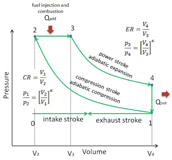
pV diagram of Carnot cycle. The area bounded by the complete cycle path represents the total work that can be done during one cycle.

See also: Carnot Cycle

In 1824, a French engineer and physicist, Nicolas Léonard Sadi Carnot advanced the study of the second law by forming a principle (also called Carnot’s rule) that specifies limits on the maximum efficiency any heat engine can obtain. In short, this principle states that the efficiency of a thermodynamic cycle depends solely on the difference between the hot and cold temperature reservoirs.

Carnot’s principle states:

  1. No engine can be more efficient than a reversible engine (a Carnot heat engine) operating between the same high temperature and low temperature reservoirs.
  2. The efficiencies of all reversible engines (Carnot heat engines) operating between the same constant temperature reservoirs are the same, regardless of the working substance employed or the operation details.

The cycle of this engine is called the Carnot cycle. A system undergoing a Carnot cycle is called a Carnot heat engine. It is not an actual thermodynamic cycle but is a theoretical construct and cannot be built in practice. All real thermodynamic processes are somehow irreversible. They are not done infinitely slowly and infinitesimally small steps in temperature are also a theoretical fiction. Therefore, heat engines must have lower efficiencies than limits on their efficiency due to the inherent irreversibility of the heat engine cycle they use.

Otto Cycle

Otto Cycle - PV Diagram
pV diagram of Otto Cycle. The area bounded by the complete cycle path represents the total work that can be done during one cycle.

See also: Otto Cycle

See also: Atkinson Cycle

The cycle of the Otto engine is called the Otto cycle. It is the one of most common thermodynamic cycles that can be found in automobile engines and describes the functioning of a typical spark ignition piston engine. In contrast to Carnot cycle, the Otto cycle does not execute isothermal processes, because these must be performed very slowly. In an ideal Otto cycle, the system executing the cycle undergoes a series of four internally reversible processes: two isentropic (reversible adiabatic) processes alternated with two isochoric processes.

Since Carnot’s principle states that no engine can be more efficient than a reversible engine (a Carnot heat engine) operating between the same high temperature and low temperature reservoirs, the Otto engine it must have lower efficiency than the Carnot efficiency. A typical gasoline automotive engine operates at around 25% to 30% of thermal efficiency. About 70-75% is rejected as waste heat without being converted into useful work, i.e. work delivered to wheels.

Diesel Cycle

Diesel cycle - pV Diagram
Diesel cycle – pV Diagram

See also: Diesel Cycle

See also: Dual Cycle

Diesel cycle is one of most common thermodynamic cycles that can be found in automobile engines and describes the functioning of a typical compression ignition piston engine. The Diesel engine is similar in operation to the gasoline engine. The most important difference is that:

  • There is no fuel in the cylinder at the beginning of the compression stroke, therefore an autoignition does not occur in Diesel engines.
  • Diesel engine uses compression ignition instead of spark ignition.
  • Because of the high temperature developed during the adiabatic compression, the fuel ignites spontaneously as it is injected. Therefore no spark plugs are needed.
  • Before the beginning of the power stroke, the injectors start to inject fuel directly into the combustion chamber and therefore first part of power stroke occurs approximately at the constant pressure.
  • Higher compression ratios can be achieved in Diesel engines, than in Otto engines

Brayton Cycle

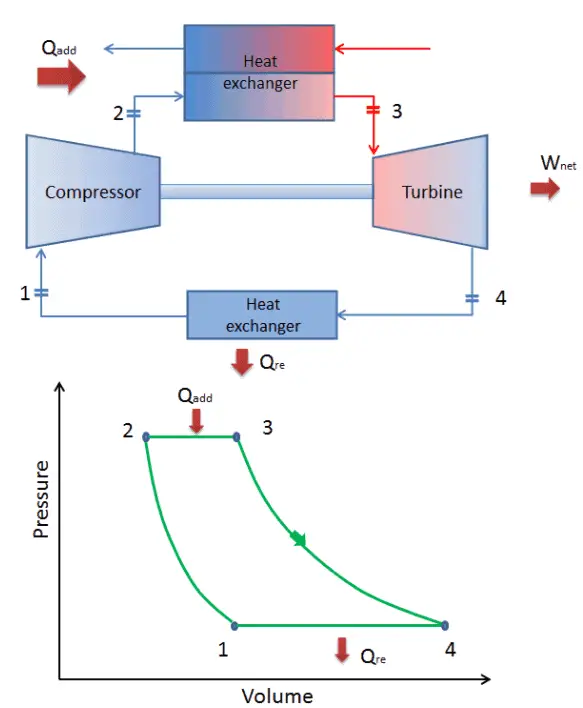
closed Brayton cycle - pV Diagram
closed Brayton cycle

See also: Brayton Cycle

See also: Ericsson Cycle

In 1872, an American engineer, George Bailey Brayton advanced the study of heat engines by patenting a constant pressure internal combustion engine, initially using vaporized gas but later using liquid fuels such as kerosene. This heat engine is known as “Brayton’s Ready Motor”. It means, the original Brayton engine used a piston compressor and piston expander instead of a gas turbine and gas compressor.

Today, modern gas turbine engines and airbreathing jet engines are also a constant-pressure heat engines, therefore we describe their thermodynamics by the Brayton cycle. In general, the Brayton cycle describes the workings of a constant-pressure heat engine.

It is the one of most common thermodynamic cycles that can be found in gas turbine power plants or in airplanes. In contrast to Carnot cycle, the Brayton cycle does not execute isothermal processes, because these must be performed very slowly. In an ideal Brayton cycle, the system executing the cycle undergoes a series of four processes: two isentropic (reversible adiabatic) processes alternated with two isobaric processes.

Rankine Cycle

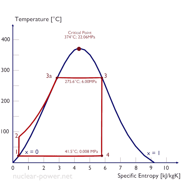
Rankine Cycle - Ts Diagram
Rankine Cycle – Ts Diagram

See also: Rankine Cycle

In 1859, a Scottish engineer, William John Macquorn Rankine advanced the study of heat engines by publishing the “Manual of the Steam Engine and Other Prime Movers”. Rankine developed a complete theory of the steam engine and indeed of all heat engines. Together with Rudolf Clausius and William Thomson (Lord Kelvin), he was a contributor to the thermodynamics, particularly focusing on the first of the three thermodynamic laws.The Rankine cycle was named after him and describes the performance of steam turbine systems, though the theoretical principle also applies to reciprocating engines such as steam locomotives. In general, the Rankine cycle is an idealized thermodynamic cycle of a constant pressure heat engine that converts part of heat into mechanical work. In this cycle the heat is supplied externally to a closed loop, which usually uses water (in a liquid and vapor phase) as the working fluid. In contrast to the Brayton cycle, the working fluid in the Rankine cycle undergo the phase change from a liquid to vapor phase and vice versa.

While many substances could be used as the working fluid in the Rankine cycle (inorganic or even organic), water is usually the fluid of choice due to its favorable properties, such as its non-toxic and unreactive chemistry, abundance, and low cost, as well as its thermodynamic properties. For example, water has the highest specific heat of any common substance –  4.19 kJ/kg K. Moreover it has very high heat of vaporization, which makes it an effective coolant and medium in thermal power plants and other energy industry. In case of the Rankine cycle, the Ideal Gas Law almost cannot be used (steam do not follow pV=nRT), therefore all important parameters of water and steam are tabulated in so called “Steam Tables“.

One of the major advantages of the Rankine cycle is that the compression process in the pump takes place on a liquid. By condensing the working steam to a liquid (inside a condenser) the pressure at the turbine outlet is lowered and the energy required by the feed pump consumes only 1% to 3% of the turbine output power and these factors contribute to a higher efficiency for the cycle.

Today, the Rankine cycle is the fundamental operating cycle of all thermal power plants where an operating fluid is continuously evaporated and condensed. It is the one of most common thermodynamic cycles, because in most of the places in the world the turbine is steam-driven.

 
References:
Nuclear and Reactor Physics:
  1. J. R. Lamarsh, Introduction to Nuclear Reactor Theory, 2nd ed., Addison-Wesley, Reading, MA (1983).
  2. J. R. Lamarsh, A. J. Baratta, Introduction to Nuclear Engineering, 3d ed., Prentice-Hall, 2001, ISBN: 0-201-82498-1.
  3. W. M. Stacey, Nuclear Reactor Physics, John Wiley & Sons, 2001, ISBN: 0- 471-39127-1.
  4. Glasstone, Sesonske. Nuclear Reactor Engineering: Reactor Systems Engineering, Springer; 4th edition, 1994, ISBN: 978-0412985317
  5. W.S.C. Williams. Nuclear and Particle Physics. Clarendon Press; 1 edition, 1991, ISBN: 978-0198520467
  6. Kenneth S. Krane. Introductory Nuclear Physics, 3rd Edition, Wiley, 1987, ISBN: 978-0471805533
  7. G.R.Keepin. Physics of Nuclear Kinetics. Addison-Wesley Pub. Co; 1st edition, 1965
  8. Robert Reed Burn, Introduction to Nuclear Reactor Operation, 1988.
  9. U.S. Department of Energy, Nuclear Physics and Reactor Theory. DOE Fundamentals Handbook, Volume 1 and 2. January 1993.

Advanced Reactor Physics:

  1. K. O. Ott, W. A. Bezella, Introductory Nuclear Reactor Statics, American Nuclear Society, Revised edition (1989), 1989, ISBN: 0-894-48033-2.
  2. K. O. Ott, R. J. Neuhold, Introductory Nuclear Reactor Dynamics, American Nuclear Society, 1985, ISBN: 0-894-48029-4.
  3. D. L. Hetrick, Dynamics of Nuclear Reactors, American Nuclear Society, 1993, ISBN: 0-894-48453-2.
  4. E. E. Lewis, W. F. Miller, Computational Methods of Neutron Transport, American Nuclear Society, 1993, ISBN: 0-894-48452-4.

See also:

Thermodynamics

We hope, this article, Thermodynamic Cycles, helps you. If so, give us a like in the sidebar. Main purpose of this website is to help the public to learn some interesting and important information about thermal engineering.
What is Carnot Cycle – Carnot Heat Engine – Definition

A system undergoing a Carnot cycle is called a Carnot heat engine. Carnot cycle is a theoretical cycle with the highest possible efficiency of all thermodynamic cycles. Thermal Engineering

Carnot Cycle – Carnot Heat Engine

pV diagram of Carnot cycle
pV diagram of Carnot cycle. The area bounded by the complete cycle path represents the total work that can be done during one cycle.

The second law of thermodynamics places constraints upon the direction of heat transfer and sets an upper limit to the efficiency of conversion of heat to work in heat engines. So the second law is directly relevant for many important practical problems.

In 1824, a French engineer and physicist, Nicolas Léonard Sadi Carnot advanced the study of the second law by forming a principle (also called Carnot’s rule) that specifies limits on the maximum efficiency any heat engine can obtain. In short, this principle states that the efficiency of a thermodynamic cycle depends solely on the difference between the hot and cold temperature reservoirs.

Carnot’s principle states:

  1. No engine can be more efficient than a reversible engine (a Carnot heat engine) operating between the same high temperature and low temperature reservoirs.
  2. The efficiencies of all reversible engines (Carnot heat engines) operating between the same constant temperature reservoirs are the same, regardless of the working substance employed or the operation details.

The cycle of this engine is called the Carnot cycle. A system undergoing a Carnot cycle is called a Carnot heat engine. It is not an actual thermodynamic cycle but is a theoretical construct and cannot be built in practice. All real thermodynamic processes are somehow irreversible. They are not done infinitely slowly and infinitesimally small steps in temperature are also a theoretical fiction. Therefore, heat engines must have lower efficiencies than limits on their efficiency due to the inherent irreversibility of the heat engine cycle they use.

Carnot Cycle – Processes

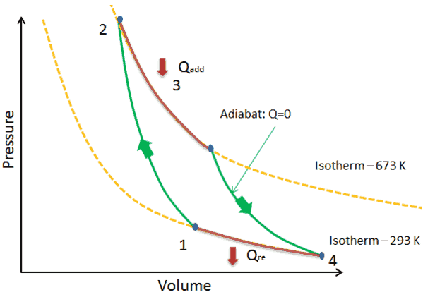
Carnot cycle - ProcessesIn a Carnot cycle, the system executing the cycle undergoes a series of four internally reversible processes: two isentropic processes (reversible adiabatic) alternated with two isothermal processes:

  1. isentropic compression – The gas is compressed adiabatically from state 1 to state 2, where the temperature is TH. The surroundings do work on the gas, increasing its internal energy and compressing it. On the other hand the entropy remains unchanged.
  2. Isothermal  expansion – The system is placed in contact with the reservoir at TH. The gas expands isothermally while receiving energy QH from the hot reservoir by heat transfer. The temperature of the gas does not change during the process. The gas does work on the surroundings. The total entropy change is given by: ∆S = S1 – S4 = QH/TH
  3. isentropic expansion – The gas expands adiabatically from state 3 to state 4, where the temperature is TC. The gas does work on the surroundings and loses an amount of internal energy equal to the work that leaves the system. Again the entropy remains unchanged.
  4. isothermal compression – The system is placed in contact with the reservoir at TC. The gas compresses isothermally to its initial state while it discharges energy QC to the cold reservoir by heat transfer. In this process the surroundings do work on the gas. The total entropy change is given by: ∆S = S3 – S2 = QC/TC

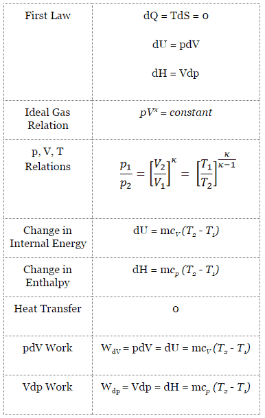
Isentropic Process

An isentropic process is a thermodynamic process, in which the entropy of the fluid or gas remains constant. It means the isentropic process is a special case of an adiabatic process in which there is no transfer of heat or matter. It is a reversible adiabatic process. The assumption of no heat transfer is very important, since we can use the adiabatic approximation only in very rapid processes.

Isentropic Process and the First Law

For a closed system, we can write the first law of thermodynamics in terms of enthalpy:

dH = dQ + Vdp

or

dH = TdS + Vdp

Isentropic process (dQ = 0):

dH = Vdp     →     W = H2 – H1     →     H2 – H1 = Cp (T2 – T1)    (for ideal gas)

Isentropic Process of the Ideal Gas

The isentropic process (a special case of adiabatic process) can be expressed with the ideal gas law as:

pVκ = constant

or

p1V1κ = p2V2κ

in which κ = cp/cv is the ratio of the specific heats (or heat capacities) for the gas. One for constant pressure (cp) and one for constant volume (cv). Note that, this ratio κ  = cp/cv is a factor in determining the speed of sound in a gas and other adiabatic processes.

Isothermal Process

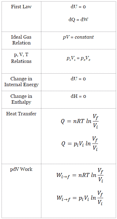
An isothermal process is a thermodynamic process, in which the temperature of the system remains constant (T = const). The heat transfer into or out of the system typically must happen at such a slow rate in order to continually adjust to the temperature of the reservoir through heat exchange. In each of these states the thermal equilibrium is maintained.

Isothermal Process and the First Law

The classical form of the first law of thermodynamics is the following equation:

dU = dQ – dW

In this equation dW is equal to dW = pdV and is known as the boundary work.

In isothermal process and the ideal gas, all heat added to the system will be used to do work:

Isothermal process (dU = 0):

dU = 0 = Q – W    →     W = Q      (for ideal gas)

Isothermal Process of the Ideal Gas

The isothermal process can be expressed with the ideal gas law as:

pV = constant

or

p1V1 = p2V2

On a p-V diagram, the process occurs along a line (called an isotherm) that has the equation p = constant / V.

See also: Boyle-Mariotte Law

Isentropic Process - characteristics
Isentropic process – main characteristics
Isothermal process - main characteristics
Isothermal process – main characteristics

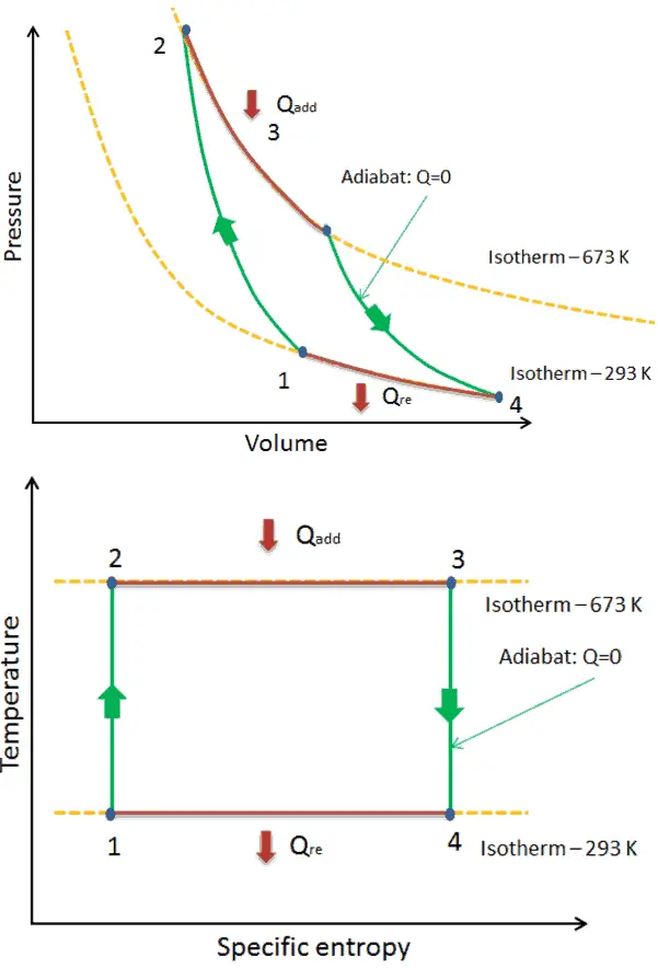
Carnot Cycle – pV, Ts diagram

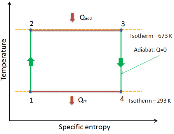
Ts diagram of Carnot cycle
Ts diagram of Carnot cycle. The area under the Ts curve of a process is the heat transferred to the system during that process.

The Carnot cycle is often plotted on a pressure- volume diagram (pV diagram) and on a temperature-entropy diagram (Ts diagram).

When plotted on a pressure-volume diagram, the isothermal processes follow the isotherm lines for the gas, adiabatic processes move between isotherms and the area bounded by the complete cycle path represents the total work that can be done during one cycle.

The temperature-entropy diagram (Ts diagram) in which the thermodynamic state is specified by a point on a graph with specific entropy (s) as the horizontal axis and absolute temperature (T) as the vertical axis, is the best diagram to describe behaviour of a Carnot cycle.

It is a useful and common tool, particularly because it helps to visualize the heat transfer during a process. For reversible (ideal) processes, the area under the T-s curve of a process is the heat transferred to the system during that process.

Carnot Cycle Efficiency

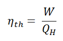
In general, the thermal efficiency, ηth, of any heat engine is defined as the ratio of the net work it does, W, to the heat input at the high temperature, QH.

thermal efficiency formula - 1

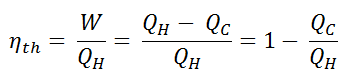
Since energy is conserved according to the first law of thermodynamics and energy cannot be be converted to work completely, the heat input, QH, must equal the work done, W, plus the heat that must be dissipated as waste heat QC into the environment. Therefore we can rewrite the formula for thermal efficiency as:

thermal efficiency formula - 2

Since QC = ∆S.TC and QH = ∆S.TH, the formula for this maximum efficiency is:

Carnot Efficiency Formula

where:

  • is the efficiency of Carnot cycle, i.e. it is the ratio = W/QH of the work done by the engine to the heat energy entering the system from the hot reservoir.
  • TC is the absolute temperature (Kelvins) of the cold reservoir,
  • TH is the absolute temperature (Kelvins) of the hot reservoir.

See also : Causes of Inefficiencies

Example: Carnot efficiency for coal-fired power plant

In a modern coal-fired power plant, the temperature of high pressure steam (Thot) would be about 400°C (673K) and Tcold, the cooling tower water temperature, would be about 20°C (293K). For this type of power plant the maximum (ideal) efficiency will be:

ηth= 1 – Tcold/Thot = 1 – 293/673 = 56%

It must be added, this is an idealized efficiency. The Carnot efficiency is valid for reversible processes. These processes cannot be achieved in real cycles of power plants. The Carnot efficiency dictates that higher efficiencies can be attained by increasing the temperature of the steam. This feature is valid also for real thermodynamic cycles. But this requires an increase in pressures inside boilers or steam generators. However, metallurgical considerations place an upper limits on such pressures. Sub-critical fossil fuel power plants, that are operated under critical pressure (i.e. lower than 22.1 MPa), can achieve 36–40% efficiency. Supercritical designs, that are operated at supercritical pressure (i.e. greater than 22.1 MPa),  have efficiencies around 43%. Most efficient and also very complex coal-fired power plants that are operated at “ultra critical” pressures (i.e. around 30 MPa) and use multiple stage reheat reach about 48% efficiency.

See also: Supercritical Reactor

 
References:
Nuclear and Reactor Physics:
  1. J. R. Lamarsh, Introduction to Nuclear Reactor Theory, 2nd ed., Addison-Wesley, Reading, MA (1983).
  2. J. R. Lamarsh, A. J. Baratta, Introduction to Nuclear Engineering, 3d ed., Prentice-Hall, 2001, ISBN: 0-201-82498-1.
  3. W. M. Stacey, Nuclear Reactor Physics, John Wiley & Sons, 2001, ISBN: 0- 471-39127-1.
  4. Glasstone, Sesonske. Nuclear Reactor Engineering: Reactor Systems Engineering, Springer; 4th edition, 1994, ISBN: 978-0412985317
  5. W.S.C. Williams. Nuclear and Particle Physics. Clarendon Press; 1 edition, 1991, ISBN: 978-0198520467
  6. Kenneth S. Krane. Introductory Nuclear Physics, 3rd Edition, Wiley, 1987, ISBN: 978-0471805533
  7. G.R.Keepin. Physics of Nuclear Kinetics. Addison-Wesley Pub. Co; 1st edition, 1965
  8. Robert Reed Burn, Introduction to Nuclear Reactor Operation, 1988.
  9. U.S. Department of Energy, Nuclear Physics and Reactor Theory. DOE Fundamentals Handbook, Volume 1 and 2. January 1993.

Advanced Reactor Physics:

  1. K. O. Ott, W. A. Bezella, Introductory Nuclear Reactor Statics, American Nuclear Society, Revised edition (1989), 1989, ISBN: 0-894-48033-2.
  2. K. O. Ott, R. J. Neuhold, Introductory Nuclear Reactor Dynamics, American Nuclear Society, 1985, ISBN: 0-894-48029-4.
  3. D. L. Hetrick, Dynamics of Nuclear Reactors, American Nuclear Society, 1993, ISBN: 0-894-48453-2.
  4. E. E. Lewis, W. F. Miller, Computational Methods of Neutron Transport, American Nuclear Society, 1993, ISBN: 0-894-48452-4.

See also:

Thermodynamic Cycles

We hope, this article, Carnot Cycle – Carnot Heat Engine, helps you. If so, give us a like in the sidebar. Main purpose of this website is to help the public to learn some interesting and important information about thermal engineering.
What is Carnot Cycle – Types of Processes – Definition

Carnot Cycle – Types of Processes. In a Carnot cycle, the system executing the cycle undergoes a series of four internally reversible processes. Thermal Engineering

Carnot Cycle – Processes

Carnot cycle - ProcessesIn a Carnot cycle, the system executing the cycle undergoes a series of four internally reversible processes: two isentropic processes (reversible adiabatic) alternated with two isothermal processes:

  1. isentropic compression – The gas is compressed adiabatically from state 1 to state 2, where the temperature is TH. The surroundings do work on the gas, increasing its internal energy and compressing it. On the other hand the entropy remains unchanged.
  2. Isothermal  expansion – The system is placed in contact with the reservoir at TH. The gas expands isothermally while receiving energy QH from the hot reservoir by heat transfer. The temperature of the gas does not change during the process. The gas does work on the surroundings. The total entropy change is given by: ∆S = S1 – S4 = QH/TH
  3. isentropic expansion – The gas expands adiabatically from state 3 to state 4, where the temperature is TC. The gas does work on the surroundings and loses an amount of internal energy equal to the work that leaves the system. Again the entropy remains unchanged.
  4. isothermal compression – The system is placed in contact with the reservoir at TC. The gas compresses isothermally to its initial state while it discharges energy QC to the cold reservoir by heat transfer. In this process the surroundings do work on the gas. The total entropy change is given by: ∆S = S3 – S2 = QC/TC

Isentropic Process

An isentropic process is a thermodynamic process, in which the entropy of the fluid or gas remains constant. It means the isentropic process is a special case of an adiabatic process in which there is no transfer of heat or matter. It is a reversible adiabatic process. The assumption of no heat transfer is very important, since we can use the adiabatic approximation only in very rapid processes.

Isentropic Process and the First Law

For a closed system, we can write the first law of thermodynamics in terms of enthalpy:

dH = dQ + Vdp

or

dH = TdS + Vdp

Isentropic process (dQ = 0):

dH = Vdp     →     W = H2 – H1     →     H2 – H1 = Cp (T2 – T1)    (for ideal gas)

Isentropic Process of the Ideal Gas

The isentropic process (a special case of adiabatic process) can be expressed with the ideal gas law as:

pVκ = constant

or

p1V1κ = p2V2κ

in which κ = cp/cv is the ratio of the specific heats (or heat capacities) for the gas. One for constant pressure (cp) and one for constant volume (cv). Note that, this ratio κ  = cp/cv is a factor in determining the speed of sound in a gas and other adiabatic processes.

Isothermal Process

An isothermal process is a thermodynamic process, in which the temperature of the system remains constant (T = const). The heat transfer into or out of the system typically must happen at such a slow rate in order to continually adjust to the temperature of the reservoir through heat exchange. In each of these states the thermal equilibrium is maintained.

Isothermal Process and the First Law

The classical form of the first law of thermodynamics is the following equation:

dU = dQ – dW

In this equation dW is equal to dW = pdV and is known as the boundary work.

In isothermal process and the ideal gas, all heat added to the system will be used to do work:

Isothermal process (dU = 0):

dU = 0 = Q – W    →     W = Q      (for ideal gas)

Isothermal Process of the Ideal Gas

The isothermal process can be expressed with the ideal gas law as:

pV = constant

or

p1V1 = p2V2

On a p-V diagram, the process occurs along a line (called an isotherm) that has the equation p = constant / V.

See also: Boyle-Mariotte Law

Isentropic Process - characteristics
Isentropic process – main characteristics
Isothermal process - main characteristics
Isothermal process – main characteristics
 
References:
Nuclear and Reactor Physics:
  1. J. R. Lamarsh, Introduction to Nuclear Reactor Theory, 2nd ed., Addison-Wesley, Reading, MA (1983).
  2. J. R. Lamarsh, A. J. Baratta, Introduction to Nuclear Engineering, 3d ed., Prentice-Hall, 2001, ISBN: 0-201-82498-1.
  3. W. M. Stacey, Nuclear Reactor Physics, John Wiley & Sons, 2001, ISBN: 0- 471-39127-1.
  4. Glasstone, Sesonske. Nuclear Reactor Engineering: Reactor Systems Engineering, Springer; 4th edition, 1994, ISBN: 978-0412985317
  5. W.S.C. Williams. Nuclear and Particle Physics. Clarendon Press; 1 edition, 1991, ISBN: 978-0198520467
  6. Kenneth S. Krane. Introductory Nuclear Physics, 3rd Edition, Wiley, 1987, ISBN: 978-0471805533
  7. G.R.Keepin. Physics of Nuclear Kinetics. Addison-Wesley Pub. Co; 1st edition, 1965
  8. Robert Reed Burn, Introduction to Nuclear Reactor Operation, 1988.
  9. U.S. Department of Energy, Nuclear Physics and Reactor Theory. DOE Fundamentals Handbook, Volume 1 and 2. January 1993.

Advanced Reactor Physics:

  1. K. O. Ott, W. A. Bezella, Introductory Nuclear Reactor Statics, American Nuclear Society, Revised edition (1989), 1989, ISBN: 0-894-48033-2.
  2. K. O. Ott, R. J. Neuhold, Introductory Nuclear Reactor Dynamics, American Nuclear Society, 1985, ISBN: 0-894-48029-4.
  3. D. L. Hetrick, Dynamics of Nuclear Reactors, American Nuclear Society, 1993, ISBN: 0-894-48453-2.
  4. E. E. Lewis, W. F. Miller, Computational Methods of Neutron Transport, American Nuclear Society, 1993, ISBN: 0-894-48452-4.

See also:

Carnot Cycle

We hope, this article, Carnot Cycle – Types of Processes, helps you. If so, give us a like in the sidebar. Main purpose of this website is to help the public to learn some interesting and important information about thermal engineering.
What is Carnot Cycle – pV, Ts diagram – Definition

Carnot Cycle – pV, Ts diagram. The Carnot cycle is often plotted on a pressure- volume diagram (pV diagram) and on a temperature-entropy diagram (Ts diagram). Thermal Engineering

Carnot Cycle – pV, Ts diagram

pV diagram of Carnot cycle
pV diagram of Carnot cycle. The area bounded by the complete cycle path represents the total work that can be done during one cycle.

The Carnot cycle is often plotted on a pressure- volume diagram (pV diagram) and on a temperature-entropy diagram (Ts diagram).

When plotted on a pressure-volume diagram, the isothermal processes follow the isotherm lines for the gas, adiabatic processes move between isotherms and the area bounded by the complete cycle path represents the total work that can be done during one cycle.

The temperature-entropy diagram (Ts diagram) in which the thermodynamic state is specified by a point on a graph with specific entropy (s) as the horizontal axis and absolute temperature (T) as the vertical axis, is the best diagram to describe behaviour of a Carnot cycle.

It is a useful and common tool, particularly because it helps to visualize the heat transfer during a process. For reversible (ideal) processes, the area under the T-s curve of a process is the heat transferred to the system during that process.

Ts diagram of Carnot cycle
Ts diagram of Carnot cycle. The area under the Ts curve of a process is the heat transferred to the system during that process.
 
References:
Nuclear and Reactor Physics:
  1. J. R. Lamarsh, Introduction to Nuclear Reactor Theory, 2nd ed., Addison-Wesley, Reading, MA (1983).
  2. J. R. Lamarsh, A. J. Baratta, Introduction to Nuclear Engineering, 3d ed., Prentice-Hall, 2001, ISBN: 0-201-82498-1.
  3. W. M. Stacey, Nuclear Reactor Physics, John Wiley & Sons, 2001, ISBN: 0- 471-39127-1.
  4. Glasstone, Sesonske. Nuclear Reactor Engineering: Reactor Systems Engineering, Springer; 4th edition, 1994, ISBN: 978-0412985317
  5. W.S.C. Williams. Nuclear and Particle Physics. Clarendon Press; 1 edition, 1991, ISBN: 978-0198520467
  6. Kenneth S. Krane. Introductory Nuclear Physics, 3rd Edition, Wiley, 1987, ISBN: 978-0471805533
  7. G.R.Keepin. Physics of Nuclear Kinetics. Addison-Wesley Pub. Co; 1st edition, 1965
  8. Robert Reed Burn, Introduction to Nuclear Reactor Operation, 1988.
  9. U.S. Department of Energy, Nuclear Physics and Reactor Theory. DOE Fundamentals Handbook, Volume 1 and 2. January 1993.

Advanced Reactor Physics:

  1. K. O. Ott, W. A. Bezella, Introductory Nuclear Reactor Statics, American Nuclear Society, Revised edition (1989), 1989, ISBN: 0-894-48033-2.
  2. K. O. Ott, R. J. Neuhold, Introductory Nuclear Reactor Dynamics, American Nuclear Society, 1985, ISBN: 0-894-48029-4.
  3. D. L. Hetrick, Dynamics of Nuclear Reactors, American Nuclear Society, 1993, ISBN: 0-894-48453-2.
  4. E. E. Lewis, W. F. Miller, Computational Methods of Neutron Transport, American Nuclear Society, 1993, ISBN: 0-894-48452-4.

See also:

Carnot Cycle

We hope, this article, Carnot Cycle – pV, Ts diagram, helps you. If so, give us a like in the sidebar. Main purpose of this website is to help the public to learn some interesting and important information about thermal engineering.